Generating a Longitudinal Dataset

This example focuses on generating a dataset to analyze determinants of health satisfaction. You can either use the syntax generator in paneldata.org or write a syntax file yourself. You can search for variable names in Paneldata.org.

In the previous examples, you created an exercise path with four subfolders as well as corresponding globals in the STATA do-file. You can use the same folders and globals for this exercise.

Create an exercise path with four subfolders:

Example:

• H:/material/exercises/do

• H:/material/exercises/output

• H:/material/exercises/temp

• H:/material/exercises/log

1.Generate an unbalanced panel dataset for the years 2006 to 2008 using paneldata.org if you wish. The dataset should contain all respondents in private households:

The data set should contain the following variables of interest:

• health satisfaction "wp0101" "xp0101" "yp0101"

• currently smoking yes/no "wp9301" "yp10601"

• current employment status "emplst06" "emplst07" "emplst08"

• monthly household net income "hinc06" "hinc07" "hinc08"

In addition, the dataset should include the following additional information for analysis from 2006 to 2008:

• cross-sectional weighting factors for all relevant years "wphrf" "xphrf" "yphrf"

• individual identifier "pid"

• original household number "cid"

• household number for all relevant years "hid_2006" "hid_2007" "hid_2008"

• sample membership "psample"

• sex "sex"

• year of birth "gebjahr"

• population membership "wpop" "xpop" "ypop"

If you need detailed instructions on how the script generator works in paneldata.org, you can find them in the chapter Syntax Generator on paneldata.org.

If you would like to assemble your dataset yourself, you can do this with the datasets you have assembled. From the previous exercise with tracking data, you may already have an idea where to get most of the variables.

Since we want to have an unbalanced panel set, the $netto variable for the years 2006 to 2008 must also be used. In addition, our analysis must limit population membership, as we are only interested in household respondents.

1.1. Create a Master File

Use ppfad as the source file together with the required variables that you may have already found in Paneldata.org or identified from the variable label in the dataset. Note that only variables from the years to be analyzed should be used.

use ypop hid_2007 cid xpop sex wnetto wpop hid_2008 xnetto pid hid_2006 psample ynetto gebjahr /// 
using "${MY_PATH_IN}ppfad.dta", clear

Since we want to obtain an unbalanced data set, i.e., individuals who have completed an individual questionnaire at least once within the last three years, you must restrict the variable $netto (survey status). Also, we only want to analyze private households, so we need a further restriction of the $pop (sample membership) variable.

* * * BALANCED VS UNBALANCED * * *

keep if ( (xnetto >= 10 & xnetto < 20) | (ynetto >= 10 & ynetto < 20) | (wnetto >= 10 & wnetto < 20) )


* * * ONLY PRIVATE HOUSEHOLDS * * *

keep if ( (xpop == 1 | xpop == 2) | (ypop == 1 | ypop == 2) | (wpop == 1 | wpop == 2) )


* * * GENDER ( male = 1 / female = 2) * * *

/* all genders */


* * * SAVE PFAD * * *

save "${MY_PATH_OUT}pfad.dta", replace 
clear

What is still missing is the cross-sectional weighting factor and the variables of interest for the analysis.

* * * HRF * * *

use cid wphrf pid yphrf xphrf prgroup /// 
using "${MY_PATH_IN}phrf.dta" 
save "${MY_PATH_OUT}hrf.dta", replace 
clear

Now we come to the content variables. In order not to have to click through all of the datasets in the data release, it is recommended that the label be entered for the variable of interest from paneldata.org.

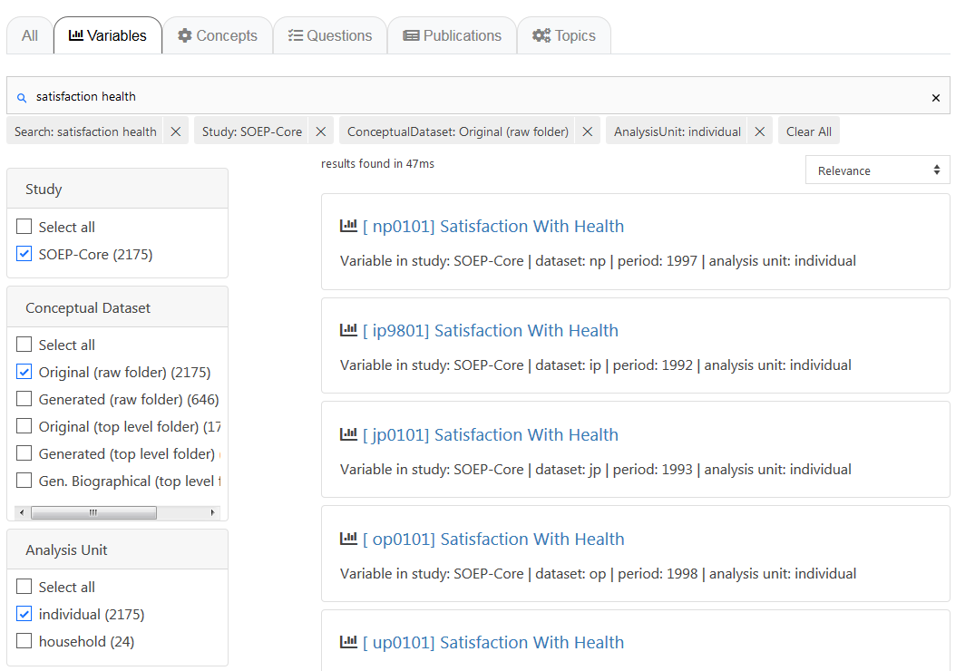
Use the filter to narrow your search. Select our main study SOEP-Core, the search type “variable”, the conceptual dataset “Original (raw folder)”, analysis unit and the corresponding year. Once you have clicked on the year of interest, a variable history is displayed. You can use this to see which years the variable was collected and what the variable is called.

Example: Variable Label “Satisfaction Health”

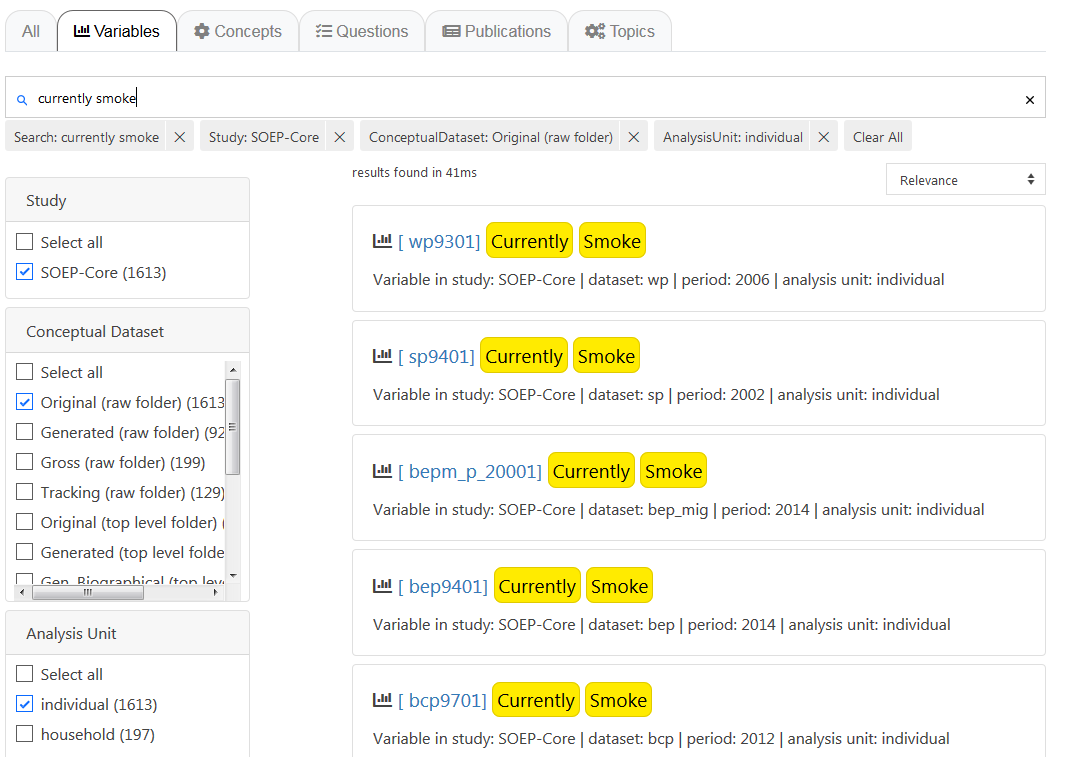
Example: Variable Label “currently smoking yes/no”

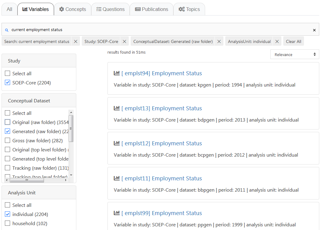
Example: Variable Label “current employment status”

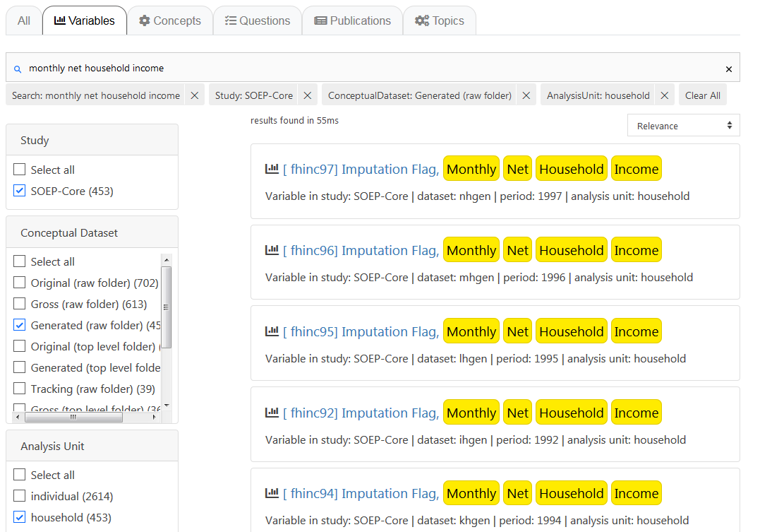
Example: Variable Label “monthly net household income”

To merge the data, you can either use the script generator on paneldata.org or write the syntax manually into a do-file.

We now have all the information we need to create a master file.

using "${MY_PATH_IN}phrf.dta" 
save "${MY_PATH_OUT}hrf.dta", replace 
clear



* * * CREATE MASTER * * *

use "${MY_PATH_OUT}pfad.dta", clear
merge 1:1 pid cid using "${MY_PATH_OUT}hrf.dta", keep(master match) nogen
save "${MY_PATH_OUT}master.dta", replace


* * * READ DATA * * *

use hinc07 hid_2007 using "${MY_PATH_IN}xhgen.dta", clear
save "${MY_PATH_OUT}xhgen.dta", replace


use xp0101 pid using "${MY_PATH_IN}xp.dta", clear
save "${MY_PATH_OUT}xp.dta", replace


use yp0101 pid yp10601 using "${MY_PATH_IN}yp.dta", clear
save "${MY_PATH_OUT}yp.dta", replace


use wp9301 pid wp0101 using "${MY_PATH_IN}wp.dta", clear
save "${MY_PATH_OUT}wp.dta", replace


use emplst07 pid using "${MY_PATH_IN}xpgen.dta", clear
save "${MY_PATH_OUT}xpgen.dta", replace


use hinc08 hid_2008 using "${MY_PATH_IN}yhgen.dta", clear
save "${MY_PATH_OUT}yhgen.dta", replace


use pid emplst06 using "${MY_PATH_IN}wpgen.dta", clear
save "${MY_PATH_OUT}wpgen.dta", replace


use hid_2006 hinc06 using "${MY_PATH_IN}whgen.dta", clear
save "${MY_PATH_OUT}whgen.dta", replace


use emplst08 pid using "${MY_PATH_IN}ypgen.dta", clear
save "${MY_PATH_OUT}ypgen.dta", replace

With the help of a unique identifier, which is either the household (hid_$) or individual identifier (pid), you can now merge all datasets or individual variables to ppfad. Which identifier to use when depends on the unit of analysis. Since we are on the individual level, our indicator is pid (individual identifier).

We load the dataset ppfad and merge our datasets or variables to ppfad.

* * * MERGE DATA * * *

use   "${MY_PATH_OUT}master.dta", clear
merge m:1 hid_2007 using "${MY_PATH_OUT}xhgen.dta", keep(master match) nogen
merge 1:1 pid using "${MY_PATH_OUT}xp.dta", keep(master match) nogen
merge 1:1 pid using "${MY_PATH_OUT}yp.dta", keep(master match) nogen
merge 1:1 pid using "${MY_PATH_OUT}wp.dta", keep(master match) nogen
merge 1:1 pid using "${MY_PATH_OUT}xpgen.dta", keep(master match) nogen
merge m:1 hid_2008 using "${MY_PATH_OUT}yhgen.dta", keep(master match) nogen
merge 1:1 pid using "${MY_PATH_OUT}wpgen.dta", keep(master match) nogen
merge m:1 hid_2006 using "${MY_PATH_OUT}whgen.dta", keep(master match) nogen
merge 1:1 pid using "${MY_PATH_OUT}ypgen.dta", keep(master match) nogen


* * * DONE * * *

label data "paneldata.org"
save "${MY_FILE_OUT}", replace
desc

log close

2. Encode missing values in system failings (STATA)!

After the master file has been created with all required information, the missing values, which can take between -1 to -8 in SOEP, must be recoded to missings. This step is important for converting a wide-format data set to a long format.

	mvdecode _all, mv(-1=. \ -2=.t \ -3=.x \ -5=.y \ -8=.z)

3. The data set is in “wide” format, i.e., additional years are displayed as additional variables (columns). For many analyses, it makes sense to convert datasets into the “long” format. In long format, additional years are displayed as additional lines. If the dataset covers three years, as in this example, there are three lines for each person. Convert the data set to long format using the STATA command reshape.!

Since these are cross-sectional variables, it can be assumed that each variable has at least one wave abbreviation, which makes the variable unique. Conversely, this means that the variables must be renamed before the reshape command.

Before renaming all original variables (e.g., from $P data sets) it must be checked whether the question and the answer categories were the same in all years (you can also look up the exact wording of the question in the corresponding questionnaire). If changes are made, the variables may have to be recoded.

*Check if original variable have changed over time
	tab1 wp0101 xp0101 yp0101
	tab1 wp9301 yp10601
	/*additionally check questionaires for exact wording*/

How you rename the variables is largely up to you. However, you should ensure that the name remains consistent over time and that the variable only differs according to the year (variable name + four-digit year suffix, e.g., zufr2006, zufr2007, zufr2008). You can rename the variables either manually, line by line, or for advanced users using a loop.

Example of manual renaming:

*rename time-variant variables
*with examples how to use loops (but can also be done "manually")
	rename wp9301 smoke2006
	rename yp10601 smoke2008
	rename wp0101 health2006
	rename xp0101 health2007
	rename yp0101 health2008
	...

Example of a loop:

	foreach  x in 6 7 8 {
		rename hinc0`x' hinc200`x'
		rename emplst0`x' emplst200`x'
		}

		
	local y=2006
	foreach w in w x y {
		rename `w'netto netto`y'
		rename `w'pop pop`y'
		rename `w'phrf phrf`y'
		local y=`y'+1
		}

3.1. The reshape command

Now that we have made all relevant preparations, you can start to convert the dataset. If you want to convert a dataset, you can do this in both directions:

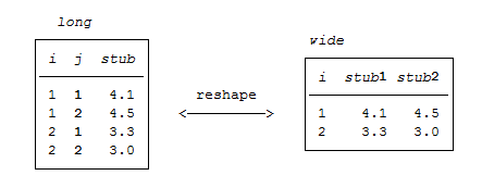
In our case, we reshape from wide to long. This means that a new variable name must be assigned for the year of the survey (j). The variable is then generated automatically. Currently, each person is assigned a line in Stata.

pid	cid	wave	sex	smoke2006	smoke2008
12345	123	x	m	yes	yes
54321	211	x	m	no	no

*reshape dataset to long-format
	reshape long health smoke emplst hinc netto pop  phrf, i(pid) j(year)
	bys pid: gen waves=_N		/*additional information: count number of waves per person*/
	tab waves

After the reshape command, you have one line per year for each person:

pid	cid	wave	year	sex	smoke
12345	123	x	2006	m	yes
12345	123	y	2007	m	.
12345	123	z	2008	m	yes

4. Perform analyses based on the data. Try to answer the following questions:

a. Has men’s and women’s average satisfaction with health changed over the three years?

Satisfaction with health was measured on a scale from 1 to 10, with a value of 10 representing the highest possible level of satisfaction. To compare the average satisfaction with health between women and men, you should display the mean value for both sexes. The mean value is displayed weighted here.

	  mean health [pw=phrf], over(sex year)

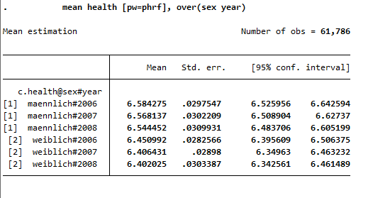
The output shows the average values for men and women for all three years. The first three values show men’s average satisfaction with health between 2006 and 2008, while the last three values show women’s average satisfaction with health.

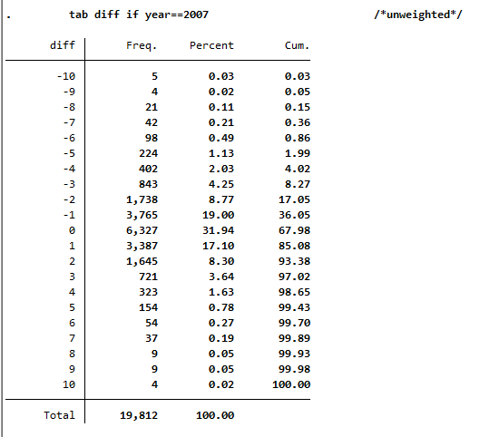
b. What is the proportion of people for whom health satisfaction has increased from 2006 to 2007?

To answer this question, the difference between 2006 and 2007 should be displayed. You should make sure that the analysis is conducted only within one persnr (individual identifier) and only for satisfaction in the following year.

	sort pid year
	gen diff=health-health[_n-1] if pid==pid[_n-1] & year==year[_n-1]+1
	tab diff if year==2007				/*unweighted*/

Since you have previously added the SOEP weighting factors to the dataset for your analysis, you should use the weighting for a representative analysis.

	tab diff if year==2007 [aw=phrf]	/*weighted*/

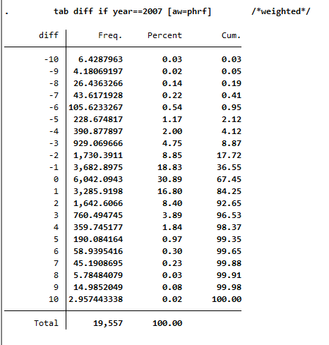
The values less than 0 show a deterioration in health satisfaction. The value 0 means constant health satisfaction, and all values above 0 show a positive change in satisfaction with their health. With a value of 10, it can be assumed that these people were interviewed for the first time in 2007 or 2008.

c. In what direction and how much has satisfaction with health changed from 2006 to 2008 among people who quit smoking after 2006?

The procedure is similar to the previous question, except that the element “smoke yes/no” is added.

	gen diff2=health-health[_n-2] if pid==pid[_n-2] & year==year[_n-2]+2 & year==2008
	gen quit=.
	replace quit=0 if smoke==1 & smoke[_n-2]==1 & pid==pid[_n-2] & year==year[_n-2]+2 & year==2008
	replace quit=1 if smoke==2 & smoke[_n-2]==1 & pid==pid[_n-2] & year==year[_n-2]+2 & year==2008
	replace quit=2 if smoke==2 & smoke[_n-2]==2 & pid==pid[_n-2] & year==year[_n-2]+2 & year==2008
	replace quit=3 if smoke==1 & smoke[_n-2]==2 & pid==pid[_n-2] & year==year[_n-2]+2 & year==2008
	label define quit 0 "smoker" 1 "quit" 2 "non-smoker" 3 "begin"
	label values quit quit
	tabstat diff2, by(quit)

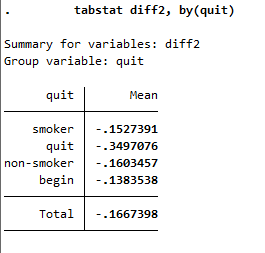
To obtain a weighted mean value, address the analysis weight after the generated variable.

	tabstat diff2 [aw=phrf], by(quit)	/*weighted*/

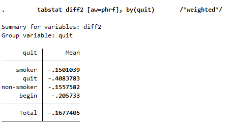
This illustration shows the mean of the health variable under the condition of the quit variable that we generated beforehand. With a mean of -0.24 (weighted -0.35), the biggest change in health satisfaction is seen in people who quit smoking after 2006. For example, if a person smoked in 2006 and indicated a satisfaction value of 8, the person indicates a satisfaction value of 7.76 after he/she stopped smoking in 2008. So you can assume that when a person stops smoking, their perceived health state deteriorates. Now we have to test if the assumption is correct.

d. Does quitting smoking make your health worse? To what extent could the result of the analysis “stop smoking” be distorted?

In order to establish a connection between health satisfaction and stopping smoking, one should use the t-test or to be more specific, the one-sample t-test. It checks whether the mean value of a sample deviates significantly from a known expected value (specified in the null hypothesis).

	* Notes: So far we have not tested whether the difference is statistically significant
		ttest diff2==0 if quit==1 		

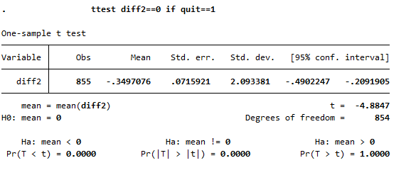
H0 Hypothesis: If one stops smoking, it has no effect on health.

For this test we assume a 95% probability. What we want to check now is whether the H0 hypothesis can be rejected or not. If you look at the output of the test, you first see the mean value of 1 (quit smoking) of the variable quit. The last line of the output shows the significance level. If it falls below the value 0.05, one can speak of a statistically significant result. In our example, the null hypothesis can be discarded because its value is less than 0.05 percent. So quitting smoking has a significant impact on a person’s perceived health.

Last change: Jun 06, 2024