Fixed Effects Estimation
Let’s say you want to find out whether certain variables relevant to the labor market, such as work experience or time in education, influence a person’s hourly wage. Other variables such as gender or marital status should also be taken into account. You decide to use the SOEP data to set up a fixed effects estimation model.
Create a path with four subfolders:

Example:
H:/material/exercises/do
H:/material/exercises/output
H:/material/exercises/temp
H:/material/exercises/log
These are used to store your script, log files, datasets, and temporary datasets. Open an empty do-file and define your paths with globals:
1***********************************************
2* Set relative paths to the working directory
3***********************************************
4global AVZ 	"H:\material\exercises"
5global MY_IN_PATH "\\hume\rdc-prod\distribution\soep-long\soep.v33.1\stata_en\"
6global MY_DO_FILES "$AVZ\do\"
7global MY_LOG_OUT "$AVZ\log\"
8global MY_OUT_DATA "$AVZ\output\"
9global MY_OUT_TEMP "$AVZ\temp\"
The global “AVZ” defines the main path. The main paths are subdivided using the globals “MY_IN_PATH”, “MY_DO_FILES”, “MY_LOG_OUT”, “MY_OUT_DATA”, “MY_OUT_TEMP”. The global “MY_IN_PATH” contains the path to your data.
a) Generate your own SOEPwage.dta dataset. The dataset should contain information on gross monthly wage, marital status, and other personal characteristics.
To perform your analysis, you need different SOEP variables. The SOEP offers various options for a variable search:
Search the questionnaires for useful variables. (For more information, see the section Variable Search with Questionnaires)
Find a suitable variable in the topic list at paneldata.org (for more information, see the section Topic Search with paneldata.org)
Search for a suitable variable using a search term in paneldata.org (for more information, see the section Variable Search with paneldata.org)
Use the documentation provided for the generated variables (for more information, seethe section Documentation on Generated Data)
Use the various important variables of the ppfadl.dta dataset as your start file. Your source file should contain the following variables:
Individual identifier "pid"
Survey year "syear"
Birth Year "gebjahr"
The net variable with information on the interview type "netto"
The weighting variable "phrf"
The gender of the person "sex"
Sample membership "pop"
1use pid syear sex gebjahr netto pop phrf using "${MY_IN_PATH}/ppfadl.dta", clear
Attention
Please note that since version 34 (v34), PPFADL has been renamed PPATHL. The following ecxercises are done with version 33.1 (v33.1), where the tracking file was named PPFADL.
Apply the necessary content variables to your starting dataset. You need the following variables for your analysis:
Employment status plb0022_h
Current gross income in euros "pglabgro"
Actual weekly working hours "pgtatzeit"
Full-time work experience "pgexpft"
Years of education or training "pgbilzeit"
Marital status in survey year "pgfamstd"
1merge 1:1 pid syear using "${MY_IN_PATH}/pl.dta", keepus(plb0022) keep(master match) nogen
2merge 1:1 pid syear using "${MY_IN_PATH}/pgen.dta", keepus(pglabgro pgtatzeit pgexpft pgbilzeit pgfamstd) keep(master match) nogen
Only keep people who have completed an interview and who live in a private household.
1* Only select people with completed interviews
2keep if inrange(netto, 10, 19)
3
4* Only private households
5keep if pop==1 | pop==2
Since you are only interested in the period from 2012 to 2016, remove all survey information that does not fall within this period. To finish, save your dataset.
1* Period from 2012 to 2016
2keep if syear>=2012 & syear<=2016
Exercise 1: Prepare your dataset
a) Load your created SOEPWage.dta dataset. It contains information on gross monthly wage, marital status, and other personal characteristics.
1*** Exercise 1: Prepare your dataset
2* a) Load data set
3use "${MY_OUT_DATA}/SOEPWage.dta", clear
b) Recode all missing values in systemmissings (.)
1* b) Recode Missings
2mvdecode _all, mv(-8/-1 = .)
For more information about the missing codes for SOEP data, see the chapter Missing Conventions
c) Generate the variables “hourly wage” (gross monthly wage/4.33*working time) for persons who have earned at least 1 euro and have worked at least one hour, “Married vs. Unmarried” and age.
1* c) Generate Variables
2gen wage = pglabgro/(4.33*pgtatzeit) if pglabgro>=1 & pgtatzeit>=1
3
4gen married = 1 if pgfamstd==1 | pgfamstd==6 | pgfamstd==7 | pgfamstd==8
5replace married = 0 if inrange(pgfamstd, 2, 5)
6
7gen age = syear - gebjahr
d) Adjust the variable “hourly wage” from outlier values by setting values smaller than the first percentile to the same value. Set values greater than 3 times the 99th percentile to 3*99th percentile. Then generate the variable lwage = log(wage).
1* d) Adjust wage variable
2sum wage, detail
3replace wage = 1/3*r(p1) if wage<1/3*r(p1)
4replace wage = 3*r(p99) if wage>3*r(p99) & wage<.
5
6gen lwage = log(wage)
7label variable lwage "Log hourly wage"
8
9save "${MY_OUT_DATA}/SOEPWage_temp.dta", replace
Exercise 2: Descriptive statistics
a) Define the dataset as a panel dataset.
1*** Exercise 2: Descriptive statistics
2* a)
3xtset pid syear // Declaring data as panel data
b) What percentage of people participated in all five waves (xtdescribe)
1* b)
2xtdescribe, patterns(16) // -> unbalanced panel
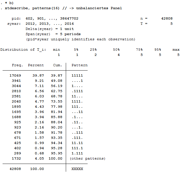
42808 respondents have contributed information within waves bc (2012) - bg (2016) and about 40% (17069) of the 42808 respondents have provided information for all waves.
c) Describe the variable “Married” with xttab and xttrans. Take a look at some individual wage (pid=30320901, pid=30932501, pid==3101602, pid==3101801) developments with xtline.
1* c)
2* Stability of the relationship status
3xttab married
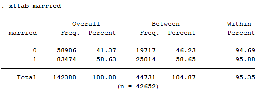
You can observe 41.37 percent of person-year observations with “married==no”. Within the period from 2012 to 2016, 19717 people responded at least once that they were not married. During the same period, 25014 persons reported at least once that they were married. Those who were not married for at least one year responded with “married==no” in 94.69% of the observations, whereas those who were married at least once responded in 95.88 percent of the observations with “married==yes”. This indicates very stable response behavior.
1* Transition probabilities
2xttrans married, freq
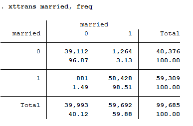
96.87 percent of the person-year observations with “married==no” are still not married in the next period. 98.51 percent of the persons who are married indicate that they will also be married in the following period. This is evidence of stable response behavior.
1* Individual sequences of "wage"
2xtline wage if pid==30320901 | pid==30932501 | pid==3101602 | pid==3101801, overlay
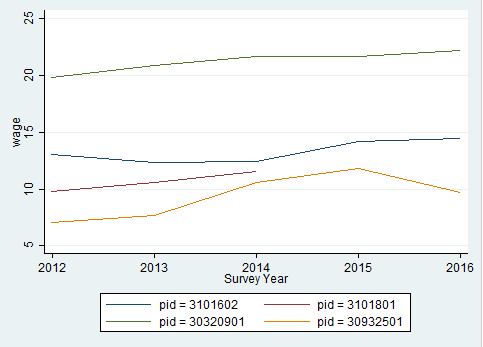
The graphic shows a comparison of the hourly wage for four different respondents.
Exercise 3: Pooled OLS Regression
a) Execute a pooled OLS regression with “log hourly wage” as dependent variable and “married”, “gender”, “work experience” and “training time” as independent variables. Interpret the coefficients for “married”, “gender” and “length of training”. Why are these not causal effects?
1*** Exercise 3: Pooled OLS Regression
2* a) Pooled OLS
3reg lwage married sex pgexpft pgbilzeit
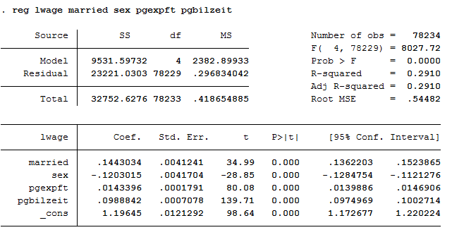
The variables married, sex, and pgbilzeit most likely correlate with other disregarded/unobserved variables that have an effect on the wage. For example, women more often work in occupations with lower wages.
b) Run the regression again with the option “vce(cluster persnr)” to get clustered standard errors. How do the standard errors of the coefficients change?
1* b) Pooled OLS with cluster standard errors
2reg lwage married sex pgexpft pgbilzeit, vce(cluster pid)
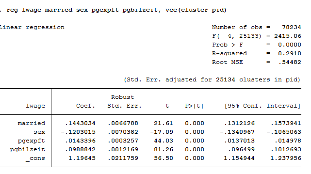
The standard errors are getting bigger.
Exercise 4: Fixed Effects
a) Subtract the person-specific mean value from each variable of the model. Use the “egen” function. Ideally you should also use a loop.
 1*** Exercise 4: Fixed Effects
 2* a) Subtract person-specific averages
 3
 4gen sample = 1
 5foreach var in lwage married sex pgexpft pgbilzeit {
 6
 7	bysort pid: egen `var'Mean = mean(`var')
 8	replace `var'Mean = . if `var'==.
 9	gen `var'Demeaned =  `var' - `var'Mean
10	replace sample = 0 if `var'==.
11}
12bysort pid (sample): replace sample = sample[1]
b) Estimate the fixed effects model with the previously generated variables. Why isn’t a coefficient estimated for “gender”? How do the coefficients change compared to the pooled OLS estimate? Is the effect of “married” now causally interpretable?
1reg lwageDemeaned marriedDemeaned sexDemeaned pgexpftDemeaned pgbilzeitDemeaned, vce(cluster pid) nocons
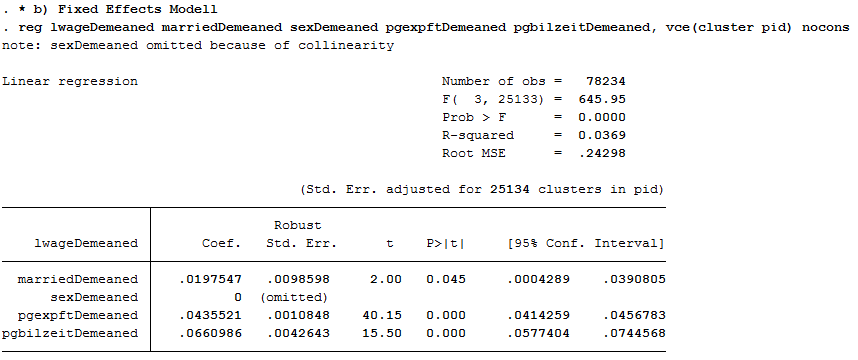
No coefficient was estimated for gender because gender was stable over time for all observations. The coefficient of married is now significant at the 5% level!
c) Now estimate the fixed effects model using the command “xtreg lwage married sex pgexpft pgbilzeit, fe”. What do you notice about the coefficients compared to task 4 b)? And with the standard errors?
1* c) xtreg, fe
2xtreg lwage married pgexpft pgbilzeit, fe vce(cluster pid)
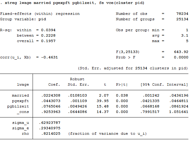
The coefficients are not identical to 4 b) and the standard errors become larger because model b) does not take into account the estimation of mean values in the standard errors.
d) Now add dummy variables for the years (i.syear). What happens to the effect of “labor market experience”?
1* d) xtreg with dummy
2xtreg lwage married pgexpft pgbilzeit i.syear, fe vce(cluster pid)
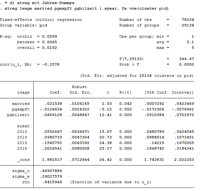
Effects on the variables remain significant. The model could possibly be specified on a case-by-case basis. The Mincer equation is based on (potential) labor market experience squared.
e) Now you can also square labor market experience into the model. To what extent does the effect of labor market experience change compared to task 5d)?
1* e) expft squared
2xtreg lwage married c.pgexpft##c.pgexpft pgbilzeit i.syear, fe vce(cluster pid)
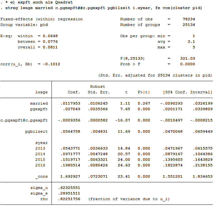
The coefficients of pgexpft and pgexpft^2 remain significant, whereas the coefficient for married is no longer significant.
1graph twoway (func y = _b[pgexpft]*x + _b[c.pgexpft#c.pgexpft]*x*x, range(0 40))
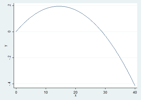
The graph shows that the effects of the labor market experience decrease after approximately 15 years of professional experience.
f) Now estimate the model from task 5e) with longitudinal section weights. Why is the number of cases now significantly smaller? Why could the coefficient of “pgbilzeit” have changed?
Tip
Create your own longitudinal person weights, e.g., longitudinal person weight from wave A to wave D. Take the starting wave cross-sectional weight (aphrf) and multiply through by each following wave staying factor, as in the following example: gen adphrf=aphrf*bpbleib*cpbleib*dpbleib
Since you are looking at the period 2012-2016, you must create a suitable longitudinal weight. To do this, use the phrf dataset from the RAW subdirectory. Apply the required variables to your analysis dataset and generate your period-related longitudinal section weight. To understand the structure of the data distribution file and the location of the different datasets, visit the section Data Distribution File. For more information about the weighting datasets and other survey datasets, see the section Survey Data.
1* f) Fixed Effects weighted
2global MY_IN_PATH2 "\\hume\rdc-prod\complete\soep-core\soep.v33.2\stata_en\"
3rename pid persnr
4merge m:1 persnr using "${MY_IN_PATH2}/phrf.dta", nogen keep(master match) keepus(bcphrf bdpbleib bepbleib bfpbleib bgpbleib)
5gen wlong = bcphrf*bdpbleib*bepbleib*bfpbleib*bgpbleib
6label variable wlong "Weighting BC-BG"
7rename persnr pid
Now estimate the model from 5e) and use the created weight.
1xtreg lwage married c.pgexpft##c.pgexpft pgbilzeit i.syear [pw=wlong], fe vce(cluster pid)
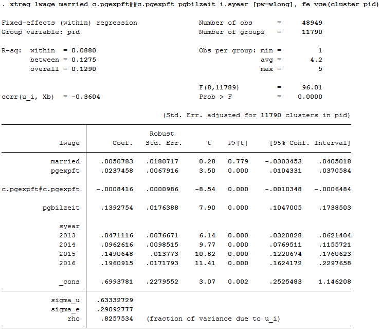
The number of observations is now much smaller. The effect of pgbilzeit is greater than before. Pgbilzeit has a lower effect in the wlong==0 group, where the return is different for each additional educational year. People in the wlong===0 group may not get the returns on additional education they expected on the local labor market and may therefore move -> higher dropout probability.
Last change: Apr 07, 2026