Working with SOEP Regional Data
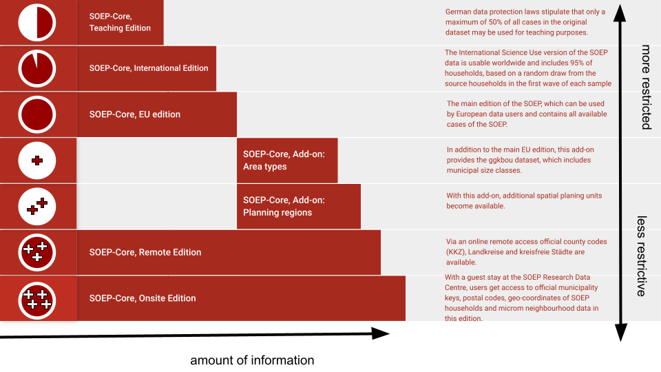
SOEP offers diverse possibilities for regional and spatial analysis. With the anonymized regional information on SOEP respondents’ (households’ and individuals’) place of residence, it is possible to link numerous regional indicators on the levels of the federal states (Bundesländer), spatial planning regions, districts, and postal codes with the data on the SOEP households. However, specific security provisions must be made due to the sensitivity of the data under data protection law. Accordingly, data users are not allowed to give any information in their analyses that could indicate, for instance, the city or district in which respondents reside. The data nevertheless provide valuable background information for regional analysis.
For more information and to access the data, see Regional Data
Assume that for your research project, you want to measure current (2016) urban-rural differences in the population. You are particularly interested in the differences in interest in politics and the different satisfaction variables provided by the SOEP. You also want to take into account demographic differences in gender and age. To be able to evaluate the potential of the data for your project, you first need an overview. For regional analysis, for example, the municipal size classes from the regional data are suitable.
Create an exercise path with four subfolders:

Example:
H:/material/exercises/do
H:/material/exercises/output
H:/material/exercises/temp
H:/material/exercises/log
These are used to store your script, log files, datasets, and temporary datasets. Open an empty do-file and define your paths with globals:
 1***********************************************
 2* Set relative paths to the working directory
 3***********************************************
 4global AVZ 	"H:\material\exercises"
 5global MY_IN_PATH "\\hume\rdc-prod\complete\soep-core\soep.v33.2\stata_en\"
 6global region "\\hume\soep-region\DATA\soep33_de\"
 7global MY_DO_FILES "$AVZ\do\"
 8global MY_LOG_OUT "$AVZ\log\"
 9global MY_OUT_DATA "$AVZ\output\"
10global MY_OUT_TEMP "$AVZ\temp\"
The global “AVZ” defines the main path. The main paths are subdivided using the globals “MY_IN_PATH”, “MY_DO_FILES”, “MY_LOG_OUT”, “MY_OUT_DATA”, “MY_OUT_TEMP”. The global “MY_IN_PATH” contains the path to the data you ordered.
a) Prepare a dataset for cross-sectional analysis covering the survey year 2016 (wave bg).
To perform your analysis, you need different SOEP variables. The SOEP offers various options for a variable search:
Search the questionnaires for useful variables (for more information, see the section Variable Search with Questionnaires)
Find a suitable variable in the topic list on paneldata.org (for more information, see the section Topic Search with paneldata.org)
Search for a suitable variable using a search term in paneldata.org (for more information, see the section Variable Search with paneldata.org)
Use the documentation provided by the generated variables (for more information, see the section Documentation on Generated Data)
Your source file should contain the following variables:
Permanent Individual ID "persnr"
Original Household Number "hhnr"
Current Wave Household Number "bghhnr"
The Sex of the Person "sex"
Year of Birth "gebjahr"
Survey Status 2016 "bgnetto"
Sample Membership 2016 "bgpop"
Weighting Factor 2016 "bgphrf"
Satisfaction With Health "bgp0101"
Satisfaction With Sleep "bgp0102"
Satisfaction With Work "bgp0103"
Satisfaction With Housework "bgp0104"
Satisfaction With Household Income "bgp0105"
Satisfaction With Personal Income "bgp0106"
Satisfaction With Dwelling "bgp0107"
Satisfaction With Amount Of Leisure Time "bgp0108"
Satisfaction With Child Care "bgp0109"
Satisfaction With Family Life "bgp0110"
Satisfaction With Social Life "bgp0111"
Satisfaction with Democracy "bgp0112"
Political Interest "bgp143"
Current Sample Region "bgsampreg"
Federal State "bgbula"
Spatial Category by BBSR "bgregtyp"
Municipal Class Sizes “ggk”
Use the key variables from the ppath.dta dataset as your starting file.
1use hhnr persnr bghhnr sex gebjahr bgnetto bgpop using ${MY_IN_PATH}\ppfad.dta, clear
Attention
Please note that since version 34 (v34), PPFAD can be found in the subdirectory “Raw” of the data distribution file. The following exercises are done with version 33.1 (v33.1), where the tracking file was named PPFAD.
Keep people who completed a questionnaire in 2016 and lived in a private household.
1* Keep people who completed a questionnaire in 2016 and live in a private household
2keep if bghhnr>0 & inrange(bgnetto, 10, 29) & inlist(bgpop, 1, 2)
3keep hhnr persnr bghhnr sex gebjahr bgnetto bgpop
4merge 1:1  persnr using ${MY_IN_PATH}\phrf.dta, keep(match master) keepusing (bgphrf) nogenerate
5tempfile ppfad
6save `ppfad'
Prepare the different datasets bgp, bghbrutto, regionl
 1* Prepare dataset bgp
 2use ${MY_IN_PATH}\bgp.dta, replace
 3keep persnr hhnr bghhnr bgp01* bgp143
 4tempfile bgp
 5save `bgp'
 6
 7* Prepare dataset bghbrutto
 8use ${MY_IN_PATH}\bghbrutto.dta, replace
 9keep hhnr bghhnr bgsampreg bgbula bgregtyp
10tempfile bghbrutto
11save `bghbrutto'
12
13* Prepare dataset regionl
14use ${region}\regionl_v33.dta, replace
15keep if syear==2016
16keep syear hhnr hhnrakt ggk
17rename hhnrakt bghhnr
18tempfile regionl
19save `regionl'
Merge all datasets.
1* Merge all datasets
2use `ppfad'
3merge 1:1 persnr using `bgp', keep(match master) nogenerate
4merge m:1 bghhnr hhnr using `regionl', keep(match master) nogenerate
5merge m:1 bghhnr hhnr using `bghbrutto', keep(match master) nogenerate
Recode negative values as missings.
1* Recode negative values into missings
2mvdecode sex gebjahr bgp01* bgp143,mv(-5/-1)
Categorize the municipal class sizes from the SOEP regional dataset.
 1* Categorize community class size
 2gen ggk_cat=.
 3replace ggk_cat=-1 if ggk==-1
 4replace ggk_cat=1 if ggk==1 | ggk==2
 5replace ggk_cat=2 if ggk==3
 6replace ggk_cat=3 if ggk==4 | ggk==5
 7replace ggk_cat=4 if ggk>5 & ggk<=7
 8
 9lab var ggk_cat "Community Size categorised"
10lab def ggk_cat -1 "No information" 1 "<=5000" 2 "5001 - 20000" 3 "20001 - 100000" ///
114 ">100000"
12lab val ggk_cat ggk_cat
Generate an age variable.
 1* Generate age variable
 2gen alter= 2016-gebjahr if gebjahr > 0
 3gen alter_cat=1 if alter<=20
 4replace alter_cat=2 if alter>20 & alter<=30
 5replace alter_cat=3 if alter>30 & alter<=65
 6replace alter_cat=4 if alter>65 & alter<=120
 7
 8lab var alter "age"
 9lab var alter_cat "age categorized"
10lab def alter_cat 1 "<=20" 2 "21-30" 3 "31-65" 4 ">65"
11lab val alter_cat alter_cat
Categorize a federal states variable.
 1* Categorize federal states
 2gen bgbula_cat=.
 3* Schleswig-Holstein + Hamburg
 4replace bgbula_cat=1 if bgbula==1 | bgbula==2
 5* Lower Saxony + Bremen
 6replace bgbula_cat=2 if bgbula==3 | bgbula==4
 7* Mecklenburg Western Pomerania + Brandenburg
 8replace bgbula_cat=3 if bgbula==13 | bgbula==12
 9* Saarland + Rhineland Palatinate
10replace bgbula_cat=4 if bgbula==7 | bgbula==10
11* Northrhine-Westphalia
12replace bgbula_cat=5 if bgbula==5
13* Hesse
14replace bgbula_cat=6 if bgbula==6
15* Baden-Württemberg
16replace bgbula_cat=7 if bgbula==8
17* Bavaria
18replace bgbula_cat=8 if bgbula==9
19* Berlin
20replace bgbula_cat=9 if bgbula==11
21* Saxony
22replace bgbula_cat=10 if bgbula==14
23* Saxony-Anhalt
24replace bgbula_cat=11 if bgbula==15
25* Thuringia
26replace bgbula_cat=12 if bgbula==16
27
28lab var bgbula_cat "Federal states categorized"
29lab def bgbula_cat 1 "Schleswig-Holstein/Hamburg" 2 "Lower Saxony/Bremen" 3 "Mecklenburg Western Pomerania/Brandenburg" ///
304 "Saarland/Rhineland Palatinate" 5 "Northrhine-Westphalia" 6 "Hesse" ///
317 "Baden-Wuerttenberg" 8 "Bavaria" 9 "Berlin" 10 "Saxony" 11 "Saxony-Anhalt" 12 "Thuringia"
32lab val bgbula_cat bgbula_cat
33drop bgbula
34rename bgbula_cat bgbula
Put the variables in your preferred order and save your dataset.
1* Order demography and identifiers first
2order persnr hhnr bghhnr syear sex gebjahr alter alter_cat bgsampreg bgbula ggk ///
3ggk_cat bgregtyp
4
5save ${MY_OUT_DATA}\zeit_online.dta, replace
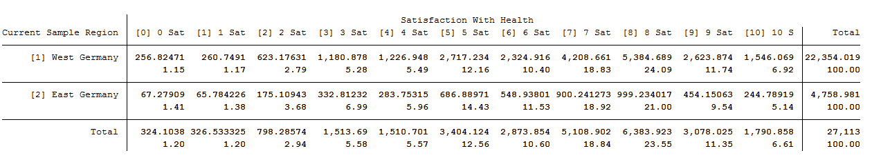
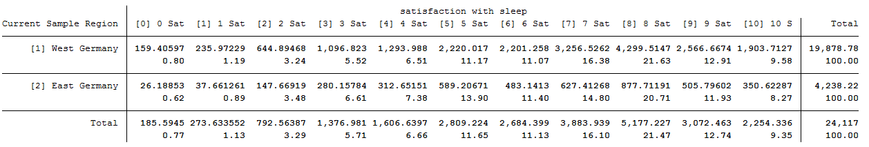
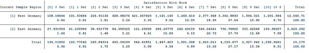
b) You want to get an initial overview of regional differences in satisfaction with various aspects of life. Use the variable bgsampreg and cross-stabilize the variable with all satisfaction variables to identify differences between East and West Germany, display the absolute and relative frequencies.
To save the tables, save them in a log file.
 1********************************************************************************
 2capture log close
 3log using "${MY_LOG_OUT}\satisfaction.log", replace
 4
 5* Life satisfaction
 6
 7local varlist bgp0101 bgp0102 bgp0103 bgp0104 bgp0105 bgp0106 bgp0107 bgp0108 ///
 8bgp0109 bgp0110 bgp0111 bgp0112
 9foreach x of local varlist {
10tab bgsampreg `x' [aw= bgphrf] , row
11}
To view all tables, look at your generated log file.
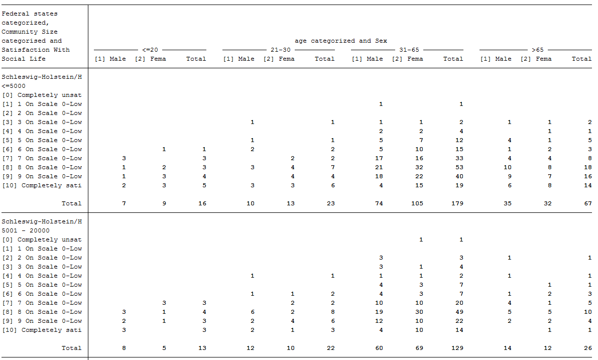
c) Now take a closer look at satisfaction with various aspects of life with the help of SOEP regional data. Use the municipal size classes. Create a table showing satisfaction with different aspects of life and highlighting differences by sex, age, municipal size class, and federal state.
1foreach x of local varlist {
2* Tabulation of satisfaction by municipal size class and federal state
3table `x' sex alter_cat, by(bgbula ggk_cat) contents(freq) column row stubwidth(20) cellwidth(8) csepwidth(2) nomissing
4* Tabulation of satisfaction by municipal size class
5table `x' sex alter_cat, by(ggk_cat) contents(freq) column row stubwidth(20) cellwidth(8) csepwidth(2) nomissing
6* Tabulation of satisfaction by federal state
7table `x' sex alter_cat, by(bgbula) contents(freq) column row stubwidth(20) cellwidth (8) csepwidth(2) nomissing
8}
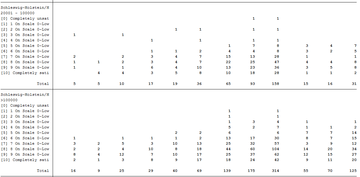
To view all tables, look at your generated log file. As you can see, SOEP regional data can be used to analyze variables at the lowest regional levels.
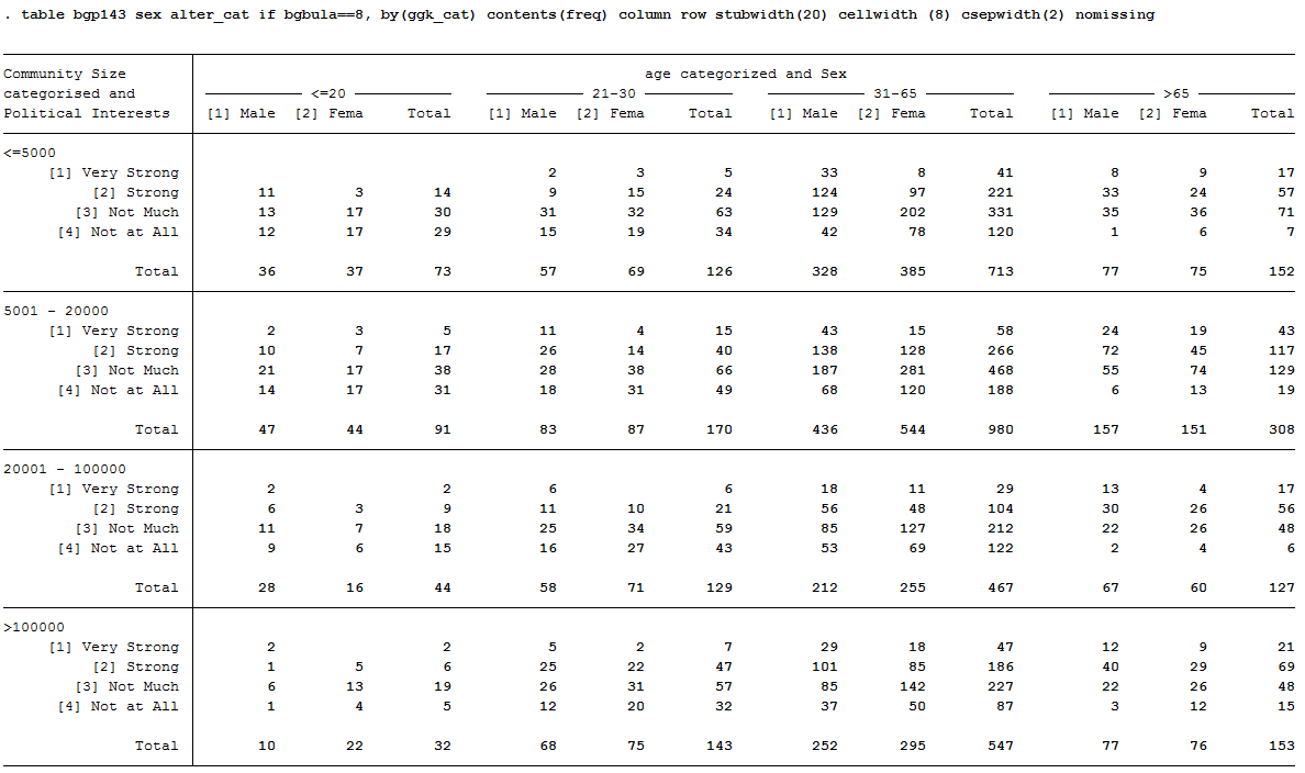
d) Create a table that shows political interest differentiated by age, sex, and municipal size class in Bavaria
1********************************************************************************
2capture log close
3log using "${MY_LOG_OUT}\political_interest.log", replace
4
5* Political interest
6* Tabulation of political interest by municipal size class for Bavaria
7table bgp143 sex alter_cat if bgbula==8, by(ggk_cat) contents(freq) column row stubwidth(20) cellwidth (8) csepwidth(2) nomissing
As you have seen here, the SOEP offers a wide range of possibilities for regional analysis. It is possible to allocate a multitude of regional indicators at the level of federal states, regional planning regions, districts, and postal codes.
Last change: Apr 07, 2026