How to Merge SOEP Data in Stata
This example focuses on merging one or more datasets for further analysis. In general, there are several ways to combine datasets:
add some extra characteristics to observations using the merge command
add some extra observations using the append command
create all pair combinations within the groups using the joinby command
In this chapter we will deal with the commands merge and joinby.
Merging two datasets requires that both have at least one variable in common (either string or numeric). This is called the key variable (for moreg information see Dataset Identifiers). Make sure that the key variables have the same notation and the same name (e.g. Person ID etc.), otherwise we will receive an error message. Examine each dataset separately before merging them. Make sure that you use all possible key variables. Depending on the data format, SOEP datasets usually have one or two key variables which can be found in the section Tracking Data in the column identifier (ID).
merge steps
Basically, for the merge you need three steps.
Open the desired dataset which is called the master dataset.
Add the second dataset which is called the using dataset.
Save the new generated dataset.
Type help merge in the STATA command line for details.
types of merges
There are three types of match merges that we frequently use.
merge 1:1
With the one-to-one merge, one observation from one dataset is matched to one observation in the other dataset. Therefore, the data are at the same level of analysis e.g. individuals to individuals. Use a unique key variable in both the master and the using datasets to merge files. Use isid in the STATA command line to find out if a variable is unique.
merge 1:m or merge m:1
In one-to-many and many-to-one merges, one observation from one dataset is matched to many observations in the other dataset. If the master dataset has many observations to match with the single observation in the using dataset, we use m:1; or we use 1:m if it is the using dataset that has many to match. e.g. households to individuals or individuals to households. One-to-many or many-to-one merges are most frequently met when dealing with hierarchical data.
_merge
After the merge the variable _merge will be automatically created. It tells us how the observations have been matched. Usually, the _merge variable has three values:
_merge == 1, observation appeared in the master file only
_merge == 2, observation appeared in the using file only
_merge == 3, observation appeared in both files
The _merge variable must be dropped or renamed before we perform the next merge.
1:1 merge - one-to-one on key variables
Compare the life satisfaction of young people between 16 and 17 years old, who were born in the German Federal States of Berlin and Hamburg.
Create an exercise path with four subfolders:

Example:
H:/material/exercises/do
H:/material/exercises/log
H:/material/exercises/output
H:/material/exercises/temp
Open an empty do-file and define your paths with globals. Globals are useful to import and export data.
1global AVZ "H:/Merge-Übung/"
2global MY_IN_PATH "//hume/rdc-prod/distribution/soep-core/soep.v37/eu/Stata/"
3global MY_DO_FILES "$AVZ/do/"
4global MY_LOG_OUT "$AVZ/log/"
5global MY_OUT_DATA "$AVZ/output/"
6global MY_OUT_TEMP "$AVZ/temp/"
First, open the desired master dataset PPATHL.
Attention
As a master data set, one uses the PPATHL or HPATHL Tracking File. The PPATHL dataset contains information on all individuals who have ever lived in a SOEP household at the point in time of a survey. The HPATHL dataset contains information on all households that have ever participated in the SOEP survey at any point in time. For more information about the data structure, see Datasets SOEP-Core .
Merge the using dataset jugendl.
Both datasets have the same level of analysis - individuals to individuals. To be able to merge both datasets, you need two identifiers to make a row in a dataset unique: pid and syear. The variable pid is the unchangeable person number. The variable syear is the year of the survey.
1use "${MY_IN_PATH}ppathl.dta", clear
2merge 1:1 pid syear using "${MY_IN_PATH}jugendl.dta"
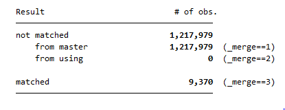
In the next step keep only the observations that are found in both datasets (_merge ==3). Delete the newly generated variable _merge.
1keep if _merge==3
2drop _merge
To answer the question we look at the variable migback, which gives the information wether an indivudual has a migration background or not. In this case we are looking for individuals who have no or an indirect migration background because the both groups were born in Germany.
1tab migback
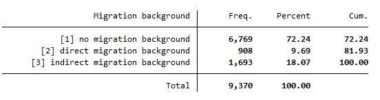
We need the values 1 and 3 for the further evaluation.
Then we look at the variable that has information about the birthplace (German Federal States). Limit the variable to the individuals who have no or an indirect migration background.
1tab birthregion if migback==1 | migback==3
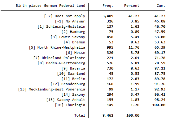
Now we know that Berlin has the value 11 and Hamburg has the value 2.
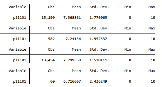
The variable jl0392 shows the life satisfaction on the scale from 0 to 10 where 10 is very satisfied and 0 is very unsatisfied. With the command sum find the mean value of the life satisfaction among the young people born in Berlin. Limit this to life satisfaction from 0 to 10 with no or an indirect migration background.
1sum jl0392 if birthregion==11 & jl0392<=10 & jl0392>=0 & ( migback==1 | migback==3 )
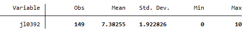
The mean value of life satisfaction in Berlin is 7.4.
Do the same for Hamburg. With the command sum find the mean value of the life satisfaction among the young people born in Hamburg. Limit this to life satisfaction from 0 to 10 with no or an indirect migration background.
1sum jl0392 if birthregion==2 & jl0392<=10 & jl0392>=0 & ( migback==1 | migback==3 )
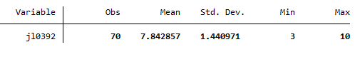
The mean value of life satisfaction in Hamburg is 7.8.
Lastly, the mean value of life satisfaction in Hamburg is 0.4 points higher than in Berlin.
1:m merge - one-to-many on key variables
Determined how life satisfaction depends on the household size in 2019.
First, open the desired master dataset HPATHL, which contains the households. Merge the using dataset PEQUIV, which is based on the Cross-National Equivalent File (CNEF) with extended income information for the SOEP. Because of different levels of analysis it is a 1:m merge. For this case, you need two key variables, hid and syear. The variable hid is the household number and the variable syear is the year of the survey. The option keep(match) keeps only the observations obtained in both datasets (or _merge==3). The option nogenerate suppresses the generation of the variable _merge.
1use "${MY_IN_PATH}hpathl.dta", clear
2merge 1:m hid syear using "${MY_IN_PATH}pequiv.dta", keep(match) nogenerate
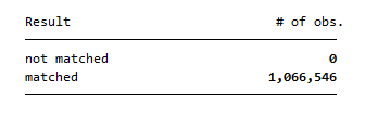
We have 1,066,546 merged observations.
Keep the observations for the survey year 2019.
1keep if syear==2019
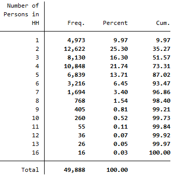
Display the variable that shows the number of persons in a household.
1tab d11106
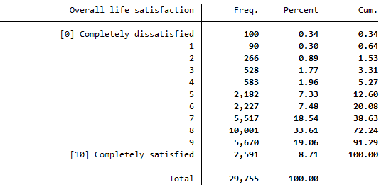
Display the life satisfaction and limit the variable from 0 to 10 where 10 is very satisfied and 0 is very dissatisfied.
1tab p11101 if p11101>=0 & p11101<=10
Sort and sum the dataset by household size. Limit the variable life satisfaction from 0 to 10.
1bysort d11106:sum p11101 if p11101>=0 & p11101<=10 & d11106==d11106
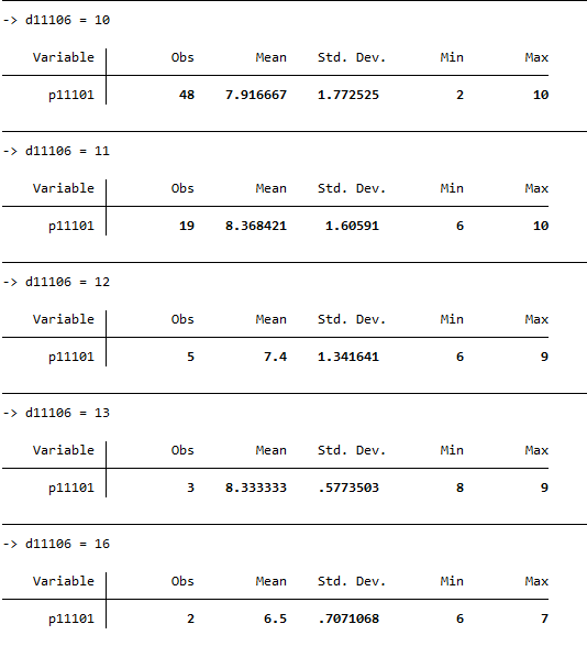
With 8.4, the highest mean score for life satisfaction is among households with 11 people. With 6.5,the lowest mean score for life satisfaction is among households with 16 people. This means that households with 11 household members are more satisfied than households with 16 people.
After the analysis save the dataset. We need it for the next exercise.
1save "${MY_OUT_DATA}hgendata.dta", replace
m:1 merge – many-to-one on key variables
Determine the extent to which life satisfaction in 2019 depends on whether the person is a main tenant, subtenant, owner or lives in a nursing home.
First, open the desired master dataset we just generated. Merge the using dataset HL, which includes all variables of the household questionnaire over time. Because of different levels of analysis it is a m:1 merge. Use two key variables hid and syear. The option keep(match) keeps only the observations obtained in both datasets (or _merge==3). The option nogenerate suppresses the generation of the variable _merge.
1use "${MY_OUT_DATA}hgendata.dta", clear
2merge m:1 hid syear using "${MY_IN_PATH}hl.dta", keep(match) nogenerate
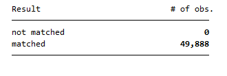
We have 49,888 merged observations.
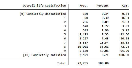
Display the variable life satisfaction limited to the 0 to 10 where 10 is very satisfied and 0 is very dissatisfied.
1tab p11101 if p11101>=0 & p11101<=10
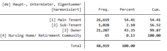
The variable hlf0001_h shows whether the individuals renting, leasing or owning the apartment or lives in a retirement home. Limit the variable to the values from 1 to 4.
1tab hlf0001_h if hlf0001_h>=1 & hlf0001_h<=4
Sum the life satisfaction for each element of the variable hlf0001_h.
1foreach hlf0001_h in 1 2 3 4 {
2sum p11101 if p11101>=0 & p11101<=10 & hlf0001_h==`hlf0001_h'
3}
Owners of apartments have the highest life satisfaction score with a mean of 7.8, while people living in nursing homes have the lowest life satisfaction score with a mean of 6.7.
After the analysis save the dataset.
1save "${MY_OUT_DATA}hlgendata.dta", replace
joinby
m:m specifies a many-to-many merge and is not a good idea. In an m:m merge, observations are matched within equal values of the key variable(s), with the first observation being matched to the first, the second, to the second, and so on. If the master and using datasets have an unequal number of observations within the group, then the last observation of the shorter group is used repeatedly to match with subsequent observations of the longer group. Thus m:m merges are dependent on the current sort order — something which should never happen. That is why you use a joinby command. joinby is similar to merge but forms all combinations of the observations where it makes sense.
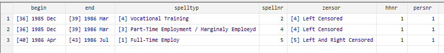
Consider the joinby command in the context of an example. For this we took segments from two datasets of the SOEP: ARTKALEN and BIOMARSM. Both are spell data. The following example is taken from the documentation “Working with spell data” , which can be downloaded here Spell Data
Open an empty do-file and define your paths with globals. Globals are useful to import and export data.
1global path "H:\Merge-Übung\examples\"
2global MY_DO_FILE "${path}example_do_files\"
3global MY_IN_PATH "${path}example_input_data\spell_to_spell\"
4global MY_OUT_PATH "${path}example_output_data\"
5global MY_TEMP_PATH "${path}example_temp_data\"
Our goal is to enrich information of one spell dataset by introducing information from the other dataset to model processes over time of two kinds. In that case, employment trajectories and their effect on the transition into marriage. We are dealing with two variables: employment status and marital status.
The ARTKALEN dataset consists of 7 variables and 3 observations. We observe only one person.
The BIOMARSM dataset consists of 7 variables and 2 observations. We also observe only one person.
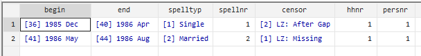
Before combining spell datasets, we prepare the two datasets separately. The preparation of both spell datasets, the master and using one, follow the exact same structure: rename variables (spelltyp to employment status and marital status), unfold each spell into subspells of duration of a single month, and delete variables we don`t need.
After preparing the dataset, ARTKALEN consists of 14 variables and 12 observations.
After preparing the dataset, BIOMARSM consists of 14 variables and 9 observations.
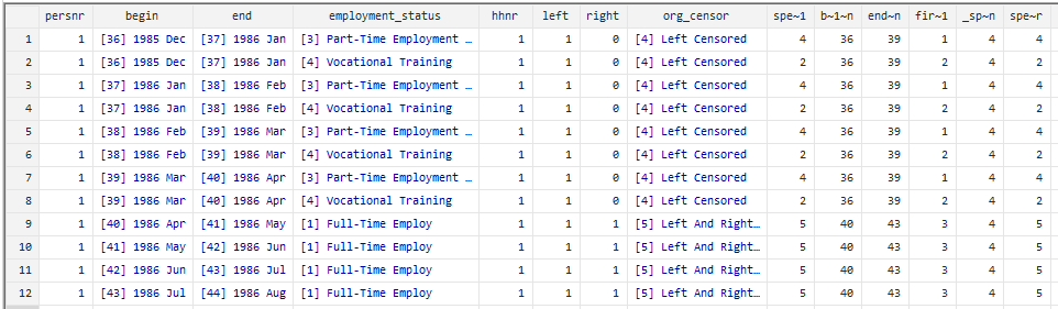
Both datasets are saved and sorted by the unique personal identification numbers and the begin date of each spell. Using both identifiers we combine the datasets.
You can see the time course and status of an individual.
1use ${MY_TEMP_PATH}\spelldata_1.dta, clear
2joinby persnr begin using ${MY_TEMP_PATH}\spelldata_2.dta, unmatched(both) update
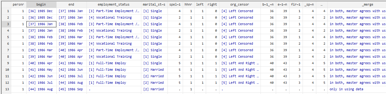
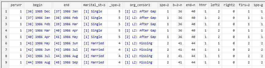
As a result, we see a combination of the first two datasets. It is about an observing person and in each row we see his employment status and marital status in a certain period of his life. In this respect we can observe how his employment status changes on the transition to marriage.
If your data has the same structure as the example, you should combine those datasets with the joinby command.