Working with spatial data in R
Prerequisites
Data Access
To work with SOEP’s spatial data you need to have a data distribution contract together with an application for stationary access to a terminal in the Research Data Center (RDC). The forms can be downloaded from here. Having data access granted, you can use the IGEL workstations in the SOEP RDC to get access to the corresponding server infrastructures MORAN and HAUSER. The MORAN server hosts the coordinates of the SOEP households together with some fake coordinates that cannot be distinguished. On this server you can, for example, compute distances or nearest points as shown later in this tutorial. On the HAUSER server you are provided your computational outcome form the MORAN server but without the coordinates. The coordinates of the SOEP households must never be available together with SOEP survey data. More information on how to use the SOEP IGEL technology can be found here.
R
When working with SOEP’s spatial data at the RDC using SOEP IGEL we
provide you with the software you need. If you want to work with spatial
test data before, you need a certain software setup. To be able to work
yourself through the following examples you need to have
R and
RStudio installed. Further, for working the
spatial data in R, you need to have GEOS, GDAL, and PROJ installed, too.
When running a Windows OS, simply install the Rtools for Windows from
here. MacOS and
Linux users are referred to the website of the sf package for
installation instructions. You can find them
here.
If you are not yet familiar with R we recommend the book R for Data Science by Wickham and Grolemund which is available here for free. Besides that, there two freely available books which are helpful to get you started with spatial data in R:
Spatial Data Science by Pebesma and Bivand which is available here
Geocomputation with R by Lovelace, Nowosad, and Muenchow which is available here
Coordinate Reference Systems
Any location of an object can be characterised by its coordinates. Besides a coordinate the altitude of an object might be of interest. So locations can be given in 2-dimensional or 3-dimensional space. A 2-dimensional coordinate referenced to two orthogonal axes (say x and y) can be given by either a pair of values (x,y) or by an angle (with respect to one of the axes) and a distance. The pair of coordinates (x,y) is referred to as cartesian coordinates and the latter as polar or spherical coordinates. In a 3-dimensional world, where you define a location on a globe, things become a little more complicated, because earth is an ellipsoid rather than a perfect sphere. In defining a location in a 3-dimensional coordinate system, the coordinate reference system (CRS) is very important. The CRS combines the information about the coordinate system itself and a geodetic datum. The geodetic datum describes how the location of the coordinate system is related to earth. So different CRS will provide different values of coordinates for the same location. Finally, the projection method provides information on how to flatten objects that are on a round surface so they can be viewed on a flat surface. The CRS is often summarised by an EPSG-code (European Petroleum Survey Group Geodesy) allowing for convenient transformations between different CRS. For more details we refer you to Chapter 2 of Spatial Data Science or Chapter 6 of Geocomputation with R. The most frequently used CRS are displayed in the following table.
EPSG code |
Note |
PRJ4-String |
Projection |
|---|---|---|---|
3857 |
WGS 84 / Pseudo-Mercator |
+proj=merc +a=6378137 +b=6378137 +lat_ts=0 +lon_0=0 +x_0=0 +y_0=0 +k=1 +units=m +nadgrids=@null +wktext +no_defs +type=crs |
Popular Visualisation Pseudo Mercator |
4326 |
WGS 84 |
+proj=longlat +datum=WGS84 +no_defs +type=crs |
(null) |
25832 |
ETRS89 / UTM zone 32N |
+proj=utm +zone=32 +ellps=GRS80 +units=m +no_defs +type=crs |
Transverse Mercator |
25833 |
ETRS89 / UTM zone 33N |
+proj=utm +zone=33 +ellps=GRS80 +units=m +no_defs +type=crs |
Transverse Mercator |
32632 |
WGS 84 / UTM zone 32N |
+proj=utm +zone=32 +datum=WGS84 +units=m +no_defs +type=crs |
Transverse Mercator |
32633 |
WGS 84 / UTM zone 33N |
+proj=utm +zone=33 +datum=WGS84 +units=m +no_defs +type=crs |
Transverse Mercator |
The differences in the maps output can be seen in the following figure. The maps show Europe (provided by https://data.opendatasoft.com) in two different CRS.
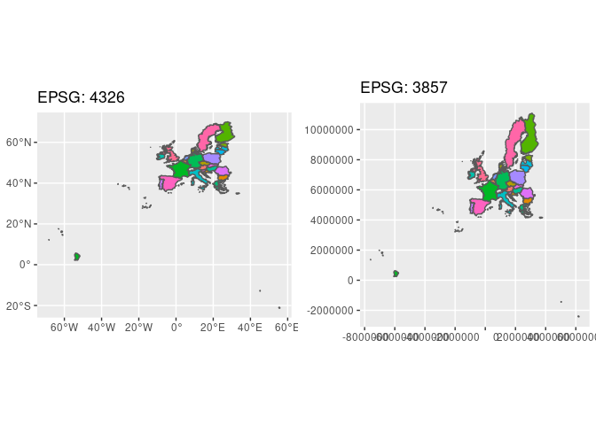
The CRS of the fake SOEP households is defined by the EPSG code 32632. The CRS usually used by Google Maps / OpenStreetMap is defined by EPSG code 4326. To check you can use for example https://coordinates-converter.com/.
If you already know about all of the prerequisites and are familiar with R, the sf package as well as the tidyverse, you can directly switch to the complete example provided in section Complete Example. If you are not familiar with all of this, we recommend you go through the following text first.
Reading data
Spatial data comes in a variety of formats, ranging from ASCII-files to more sophisticated data structures like shapefiles or XML-dialects. Fortunately the R package sf provides functions to conveniently read most of the data formats. Besides that, the package and its use is well documented here. The package can easily be installed and loaded by using the following lines of code in R.
install.packages('sf') # installing the package
library(sf) # loading the package

# further packages
install.packages('tidyverse') # a selection of packages
library(tidyverse) # (mainly using dplyr, ggplot2)
install.packages('here') # for working with .RProj and paths
library(here)
Further packages that are useful when working with R are the tidyverse (a selection of several packages) and here (makes working in projects easier). A complete list of packages used to create this page is provided in Appendix at the end of this page.
When working with spatial data in the SOEP we provide you with fake
coordinates of the SOEP households in a shapefile format. This format is
easy to read using the sf package in R and provides you with all the
details you need. The data you bring along is likely to be in a
different format. Formats that can be read using st_read are listed
in the GDAL
Documentation. If you
bring along data in other formats consider the
haven
package for SAS, SPSS, or Stata formats, documented
here. Non-spatial data formats
however, mostly include no information on the CRS. Thus you need to know
and assign it to the data. An example when reading data from
spreadsheets is provided below.
Shapefiles
Shapefiles consist of at least three files, namely
.shpcontaining the geometries for example for a point (address) or a polygon (state).dbfcontaining the attribute data for each geometry, for exampe, the address data (street, zip code, city) or names of the states.shxcontaining the indices linking geometries and attribute data
There are usually some more files provided containing further
information. One example of shapefiles is provided by the Federal Agency
for Cartography and Geodesy (BKG,
GeoBasis-DE / BKG 2019). The BKG provides public available data on
administrative areas in Germany. The dataset VG250 includes theses
administrative units of the hierarchical levels from the country down to
municipalities and is available
here.
Unzipping the folder will provide you with the shapefiles and the
documentation of the data. Because the data contains information on
different levels (Germany, its states, district, municipalities) these
are stored in different layers. To check which information is avaialable
in the data, use st_layers. If you do not explicitly provide a
layer, st_read will take the first available layer. The function
returns the layer names, the according type of geometry, the number of
features (geometries) and fields (variables). Reading the German Federal
States you need to pick the layer VG250_LAN.
# layers in the data
st_layers(here('Daten', 'vg250_ebenen_0101'))
## Driver: ESRI Shapefile
## Available layers:
##    layer_name geometry_type features fields
## 1   VG250_GEM       Polygon    11135     26
## 2   VG250_KRS       Polygon      431     26
## 3   VG250_LAN       Polygon       35     26
## 4    VG250_LI   Line String    35483      4
## 5    VG250_PK         Point    11003     13
## 6   VG250_RBZ       Polygon       20     26
## 7   VG250_STA       Polygon       11     26
## 8   VG250_VWG       Polygon     4688     26
## 9    VG_DATEN            NA       35      8
## 10   VG_WERTE            NA       32      4
# read the shapefile for Federal States
States <- st_read(here('Daten', 'vg250_ebenen_0101'), layer = 'VG250_LAN', quiet = TRUE)
Taking a look at a the main variables GEN (Geographical name),
BEZ (Designation), and geometry (a multipolygon), we are
provided with information displayed differently from usual
data.frame or tibble like data. The ‘header’ tells you it’s a
collection of simple features having 16 features (rows) and 2 fields
(variables, excluding the geometry column). The type of geomtry is a
multipolygon (set of polygons) in a two-dimensional space (XY). The
bounding box (bbox) provides information on the bottom left and top
right corner of the box bounding the geometries. Finally, you get
information on the coordinate reference system (CRS), summarized by
EPSG-Code 25832.
# look at the data
States %>%
  filter(GF == 4) %>% # use land with structure only
  select(GEN, BEZ, geometry) # select necessary variables
## Simple feature collection with 16 features and 2 fields
## geometry type:  MULTIPOLYGON
## dimension:      XY
## bbox:           xmin: 280371.1 ymin: 5235856 xmax: 921292.4 ymax: 6101444
## projected CRS:  ETRS89 / UTM zone 32N
## First 10 features:
##                    GEN                  BEZ                       geometry
## 1   Schleswig-Holstein                 Land MULTIPOLYGON (((464810.7 61...
## 2              Hamburg Freie und Hansestadt MULTIPOLYGON (((578219 5954...
## 3        Niedersachsen                 Land MULTIPOLYGON (((479451.1 59...
## 4               Bremen     Freie Hansestadt MULTIPOLYGON (((466930.3 58...
## 5  Nordrhein-Westfalen                 Land MULTIPOLYGON (((477607.3 58...
## 6               Hessen                 Land MULTIPOLYGON (((534242 5721...
## 7      Rheinland-Pfalz                 Land MULTIPOLYGON (((416304.5 56...
## 8    Baden-Württemberg                 Land MULTIPOLYGON (((546771.2 55...
## 9               Bayern            Freistaat MULTIPOLYGON (((609387.6 52...
## 10            Saarland                 Land MULTIPOLYGON (((359841 5499...
SOEP Regional Data
Also the fake coordinates for the SOEP households are provided in a
shapefile format. The data contains an ID-variable (ID) and the
survey year (erhebj) together with a point geometry. The ID
provided is not related to any of the SOEP’s hid or pid. It is
simply a number ranging from 1 to the corresponding number of rows in
the data set. Households can thus only be identified, merged, or
selected using their coordinate. Moreover the data also contain the
SOEP’s initial sample. Thus containing regional information on
respondents and non-respondents. Because of data protection regulations,
the SOEP survey data must not be used together with the household’s
coordinates. This is why the environment where you are allowed to work
with the household’s coordinates is strictly separated. Unlike the
VG250 data the SOEP data has the EPSG-code 32632.
SOEP <- st_read(here('Daten', 'soep_v29'))
## Reading layer `soep_hh_korr_nur_fakes_utm32-v29' from data source `/media/H/Projekte/Adhoc_Analysen/GeodatenBSP/Daten/soep_v29' using driver `ESRI Shapefile'
## Simple feature collection with 209734 features and 2 fields
## geometry type:  POINT
## dimension:      XY
## bbox:           xmin: 288107 ymin: 5250939 xmax: 888152 ymax: 6055336
## projected CRS:  WGS 84 / UTM zone 32N
SOEP
## Simple feature collection with 209734 features and 2 fields
## geometry type:  POINT
## dimension:      XY
## bbox:           xmin: 288107 ymin: 5250939 xmax: 888152 ymax: 6055336
## projected CRS:  WGS 84 / UTM zone 32N
## First 10 features:
##    erhebj ID               geometry
## 1    2000  1 POINT (355929 5665928)
## 2    2000  2 POINT (800240 5821852)
## 3    2000  3 POINT (794464 5831012)
## 4    2000  4 POINT (478831 5431318)
## 5    2000  5 POINT (799318 5825023)
## 6    2000  6 POINT (794752 5833726)
## 7    2000  7 POINT (799149 5824960)
## 8    2000  8 POINT (791594 5827687)
## 9    2000  9 POINT (791657 5827422)
## 10   2000 10 POINT (792280 5826345)
Spreadsheets
When reading spatial data from spreadsheets the data is read by
different drivers. The example data is contained in an Excel spreadsheet
with three variables X (longitude), Y (latitude), and
Object. Using the st_read function the csv-driver from GDAL is
chosen automatically, reading 4 columns however. Thus we get rid of the
last column first.
POI <- st_read(here('Daten', 'POIs_Berlin.csv'))
## Reading layer `POIs_Berlin' from data source `/media/H/Projekte/Adhoc_Analysen/GeodatenBSP/Daten/POIs_Berlin.csv' using driver `CSV'
POI
##                   X                Y                    Objekt field_4
## 1  13.3776978296166 52.5162788298363         Brandenburger Tor    <NA>
## 2  13.3693019102667 52.5250274843424              Hauptbahnhof    <NA>
## 3  13.3886070846104 52.5121727411876                DIW Berlin    <NA>
## 4  13.4589278721678  52.496825784817              Mulecule Man    <NA>
## 5  13.2887256012712 52.5580119710438           Flughafen Tegel    <NA>
## 6  13.4005469632413 52.4792779435797          Tempelhofer Feld    <NA>
## 7  13.4484578382279 52.4482123689564          Hufeisensiedlung    <NA>
## 8   13.281110837709 52.4473851451014                 FU Berlin    <NA>
## 9  13.1725456943567 52.4300072503147                   Wannsee    <NA>
## 10 13.2128459704725 52.5411476127425         Zitadelle Spandau    <NA>
## 11 13.5727300494297 52.4438163134271          Schloss Köpenick    <NA>
## 12 13.2795658406826 52.5080182126806 Zentraler Omnibus Bahnhof    <NA>
POI <- POI[, -4]
Because this data contains latitude and longitude already, we can simply
transform it to a spatial dataset using st_as_sf and the CRS has to
be assigned to it.
POI <- st_as_sf(POI, coords = c("X", "Y"), crs = 4326)
POI
## Simple feature collection with 12 features and 1 field
## geometry type:  POINT
## dimension:      XY
## bbox:           xmin: 13.17255 ymin: 52.43001 xmax: 13.57273 ymax: 52.55801
## geographic CRS: WGS 84
## First 10 features:
##               Objekt                  geometry
## 1  Brandenburger Tor  POINT (13.3777 52.51628)
## 2       Hauptbahnhof  POINT (13.3693 52.52503)
## 3         DIW Berlin POINT (13.38861 52.51217)
## 4       Mulecule Man POINT (13.45893 52.49683)
## 5    Flughafen Tegel POINT (13.28873 52.55801)
## 6   Tempelhofer Feld POINT (13.40055 52.47928)
## 7   Hufeisensiedlung POINT (13.44846 52.44821)
## 8          FU Berlin POINT (13.28111 52.44739)
## 9            Wannsee POINT (13.17255 52.43001)
## 10 Zitadelle Spandau POINT (13.21285 52.54115)
Transformations
To be able to work with all three data sets (States, SOEP, and
POI) we have to make sure all have the same CRS. Using
st_transform we can reproject the data sets to have the same
EPSG-code (common_crs).
common_crs <- 25832

SOEP <- st_transform(SOEP, crs = common_crs)
SOEP <- SOEP[SOEP$erhebj == 2005, ] # only use 2005 SOEP data

POI <- st_transform(POI, crs = common_crs)

# States <- st_transform(States, crs = common_crs) aleady correct crs
Sometimes it might be easier for you to work in other programs and you
wish to have latitude and longitude data. In this case you can use
st_coordinates to transform point geometries into (x,y) coordinates.
The below example first transforms the coordinates for the households 1
to 5 in the SOEP data into latitude and longitude data and then
creates the (x,y) coordinates from the point geometry.
soep5_lat_lon <-  st_transform(SOEP[1:5,], 4326)
st_coordinates(soep5_lat_lon)
##          X        Y
## 1  6.94659 51.12465
## 2 13.36828 52.48428
## 3 13.40601 52.39064
## 4  8.70727 49.03966
## 5 13.43205 52.48811
Plotting Spatial Data
Besides being able to look up coordinates or objects in google maps or
OpenStreetMap, we can use the ggplot2 package included in the
tidyverse package for displaying the data. The package provides the
geom_sf function to easily plot the data.
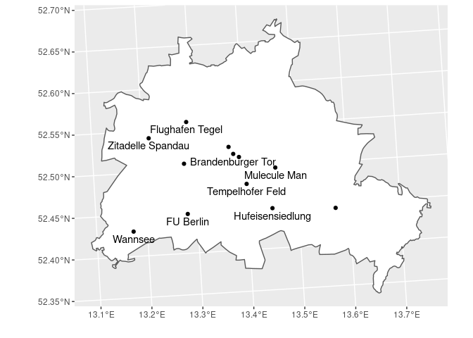
# subsetting and plotting the data
States %>% # use the states data
  filter(GEN == 'Berlin') %>% # filter for Berlin only
  ggplot() + # plot base
  geom_sf(fill = 'white') + # add the polygon for Berlin and fill it whtie
  geom_sf(data = POI) + # add the POI data
  geom_sf_text(data = POI, aes(label = Objekt),
               nudge_y = -1000,
               check_overlap = TRUE) + # overlapping labels will not be displayed
  xlab('') + ylab('')
Frequently Used Operations
This section will provide an overview of some frequently used operations
when working with spatial data. The dataset SOEP contains some fake
coordinates of household addresses we will work with throughout the
examples.
Finding Households in a Specified Area
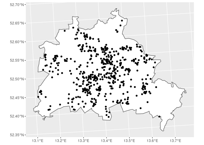
Suppose we are interested in identifying all the SOEP households located
in Berlin. The corresponding polygon for Berlin is provided in the
States dataset. Because we are interested in Berlin only, we save
the polygon in an own object BE. The function st_contains
identifies the row-index in the SOEP dataset that fall within the
polygon BE and returns a list (soep_in_berlin). For checks along
the way we can look at plots of the data.
BE <- States[States$GEN == 'Berlin', ]
BE %>% select(GEN, BEZ)
## Simple feature collection with 1 feature and 2 fields
## geometry type:  MULTIPOLYGON
## dimension:      XY
## bbox:           xmin: 777974.1 ymin: 5808837 xmax: 823510.5 ymax: 5845580
## projected CRS:  ETRS89 / UTM zone 32N
##       GEN  BEZ                       geometry
## 11 Berlin Land MULTIPOLYGON (((802831.7 58...
soep_in_berlin <- st_contains(BE, SOEP)
soep_in_berlin
## Sparse geometry binary predicate list of length 1, where the predicate was `contains'
##  1: 2, 3, 5, 6, 8, 9, 10, 11, 12, 13, ...
SOEP_BE <- SOEP[unlist(soep_in_berlin), ]

BE %>%
  ggplot() + geom_sf(fill = 'white') + geom_sf(data = SOEP_BE)
Distances / Areas
To compute distances the function st_distance can be provided a
single dataset with n rows providing a n x n matrix of distances of the
geometries contained in the data (dist_m). The unit of the distance
returned depends on the CRS. In the example provided below the distances
of the POIs to the location of the DIW are given in meters.
Providing the function a second dataset of m rows will create a n x m
distance matrix (dist_soep_poi). The created object is a matrix with
529 rows (SOEP households in Berlin) and 12 columns (POIs in Berlin).
When computing distances on large data sets it might be helpful to
subset the data, because the distance of a household in Munich might be
irrelevant to a research question focusing on Berlin or distances
smaller than 5000m. According the the CRS, consider specifying the
which argument.
Areas can be computed for (multi-)polygons. The function st_area
provides the corresponding information.
# distances between the POIs
dist_m <- st_distance(POI)
rownames(dist_m) <- POI$Objekt
colnames(dist_m) <- POI$Objekt

# distance of POIs to DIW Berlin
dist_m['DIW Berlin', ]
## Units: [m]
##         Brandenburger Tor              Hauptbahnhof                DIW Berlin
##                  870.8119                 1941.2940                    0.0000
##              Mulecule Man           Flughafen Tegel          Tempelhofer Feld
##                 5074.7951                 8488.2154                 3751.7696
##          Hufeisensiedlung                 FU Berlin                   Wannsee
##                 8202.7627                10269.1064                17307.5100
##         Zitadelle Spandau          Schloss Köpenick Zentraler Omnibus Bahnhof
##                12364.7837                14651.8215                 7422.6480
# distance between each household and each POI
dist_soep_poi <- st_distance(SOEP_BE, POI)
dim(dist_soep_poi)
## [1] 529 12
# save distances in an object
DIST <- as_tibble(dist_soep_poi)
# add names
names(DIST) <- str_c('distance_to_', str_remove(POI$Objekt, ' '))

# attach distances to data
SOEP_BE <- bind_cols(SOEP_BE, DIST)


# area covered by Berlin
st_area(BE)
## 893060962 [m^2]
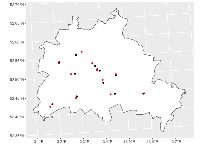
Nearest Point
To find the point or feature closest to another one the function
st_nearest_feature will return a vector with indices of the nearest
feature. In the example below we are looking for the households living
closest to the POIs in Berlin. In the second step we compute the
corresponding distances between the POI and the household.
nearest_hh <- st_nearest_feature(POI, SOEP_BE)

diag(st_distance(POI, SOEP_BE[nearest_hh, ]))
## Units: [m]
##  [1]  256.5810 1195.8833  789.6812  392.5787 1913.8130  891.4404 1295.8621
##  [8]  520.3830  971.0417  364.4532  250.2833 1194.7832
BE %>% # polygon for Berlin
  ggplot() + geom_sf(fill = 'white') + # plot the Berlin polygon
  geom_sf(data = POI) + # add the POIs
  geom_sf(data = SOEP_BE[nearest_hh, ], col = 'red') # add the nearest household
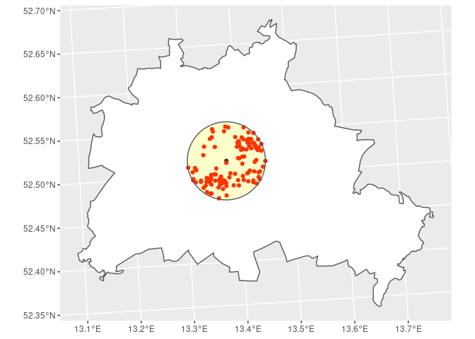
Within Distance
If your interest is about which households live within a certain
distance to a specific point, st_is_within_distance lets you lookup
geometries in a given distance (argument dist) and returns a list.
The below example looks up households in a 5km distance of the
Brandenburger Tor. The plot shows the 5km radius area in yellow, the
location of the Brandenburger Tor (black dot) and than households within
the distance (red dots).
r_5000 <- st_is_within_distance(POI[POI$Objekt == 'Brandenburger Tor',],
                                SOEP_BE,
                                dist = 5000)
r_5000
## Sparse geometry binary predicate list of length 1, where the predicate was `is_within_distance'
##  1: 1, 3, 6, 12, 21, 25, 28, 39, 54, 55, ...
BE %>% # polygon for Berlin
  ggplot() + geom_sf(fill = 'white') + # plot the Berlin polygon
  geom_sf(data = POI[POI$Objekt == 'Brandenburger Tor',]) + # add the POI
  geom_sf(data = SOEP_BE[unlist(r_5000), ], col = 'red') + # add the nearest household
  geom_sf(data = st_buffer(POI[POI$Objekt == 'Brandenburger Tor',], dist = 5000),
          alpha = 0.2, fill = 'yellow')
The question cal also be asked the other way around: How many POIs are
within a 5km radius of the SOEP households? This way the function
st_is_within_distance returns a list of length equal to the number
of SOEP households in Berlin (529). For each household the (row) index
for the POI is given. To get the number of POIs in the 5km radius, we
can simply ask for the length (the number of row indices) of each
list-component. To get the according distances see section Distances /
Areas
poi_5000 <- st_is_within_distance(SOEP_BE, POI, dist = 5000)
poi_5000
## Sparse geometry binary predicate list of length 529, where the predicate was `is_within_distance'
## first 10 elements:
##  1: 1, 2, 3, 6
##  2: (empty)
##  3: 1, 3, 4, 6, 7
##  4: 5
##  5: 2, 5, 12
##  6: 1, 2, 12
##  7: 10
##  8: 5, 10, 12
##  9: 8
##  10: 5, 10, 12
N_POI <- as_tibble(sapply(poi_5000, length))
names(N_POI) <- 'n_poi_in_5km'

SOEP_BE <- bind_cols(SOEP_BE, N_POI)
Spatial joins
When you are used to working with SOEP data you will have probably
merged / joined data sets using the identifying variables (cid,
hid, pid) and the survey year (syear) before. When you are
working with spatial data you will have to choose one of the geometry
predicate function provided by the sf package. The default is a left
join of the two data sets using st_intersects as the geometry
predicate function for joining. You can however change this, for
example, to join the nearest features, see section Nearest Point. In
our example here, we join the nearest SOEP household to each of the
points of interest. The geometry column here provides the coordinates
from the POI data set.
NEAR <- st_join(POI, SOEP, join = st_nearest_feature)
NEAR
## Simple feature collection with 12 features and 3 fields
## geometry type:  POINT
## dimension:      XY
## bbox:           xmin: 783630.5 ymin: 5817059 xmax: 810721.7 ymax: 5831749
## projected CRS:  ETRS89 / UTM zone 32N
## First 10 features:
##               Objekt erhebj    ID                 geometry
## 1  Brandenburger Tor   2005 75759 POINT (796986.8 5827473)
## 2       Hauptbahnhof   2005 69076 POINT (796358.6 5828411)
## 3         DIW Berlin   2005 75759 POINT (797754.3 5827062)
## 4       Mulecule Man   2005 75646 POINT (802628.5 5825649)
## 5    Flughafen Tegel   2005 73266 POINT (790677.7 5831749)
## 6   Tempelhofer Feld   2005 69820 POINT (798787.2 5823455)
## 7   Hufeisensiedlung   2005 69477 POINT (802251.6 5820202)
## 8          FU Berlin   2005 67568 POINT (790892.2 5819422)
## 9            Wannsee   2005 67923 POINT (783630.5 5817059)
## 10 Zitadelle Spandau   2005 68827 POINT (785646.9 5829572)
Export Results
To export your results you can use st_write to create a .csv
file. When exporting your results pleace check the requirements
here.
path_export <- paste0('/home/', Sys.info()['user'], '/transfer/export/',  Sys.Date())

if(!file.exists(path_export)){
  dir.create(path_export, recursive = TRUE)
}

st_write(SOEP_BE, file.path(path_export, 'Output_SOEP_BE.csv'),
         append = FALSE, overwrite = TRUE)

README <- tibble(name = names(SOEP_BE)[-grep('geometry', names(SOEP_BE))],
                 description = c('erhebj',
                                 'ID',
                                 'distance (in meters) of household to Brandenburger Tor',
                                 'distance (in meters) of household to Hauptbahnhof',
                                 'distance (in meters) of household to DIW-Berlin',
                                 'distance (in meters) of household to Mulecule Man',
                                 'distance (in meters) of household to Flughafen Tegel',
                                 'distance (in meters) of household to Tempelhofer Feld',
                                 'distance (in meters) of household to Hufeisensiedlung',
                                 'distance (in meters) of household to FU Berlin',
                                 'distance (in meters) of household to Wannsee',
                                 'distance (in meters) of household to Zitadelle Spandau',
                                 'distance (in meters) of household to Schloss Köpenick',
                                 'distance (in meters) of household to Zentraler Omnibus Bahnhof',
                                 'number of POIs within 5 km radius of household'))

write.csv(README, file.path(path_export, 'Output_SOEP_BE.csv'),
         row.names = FALSE)
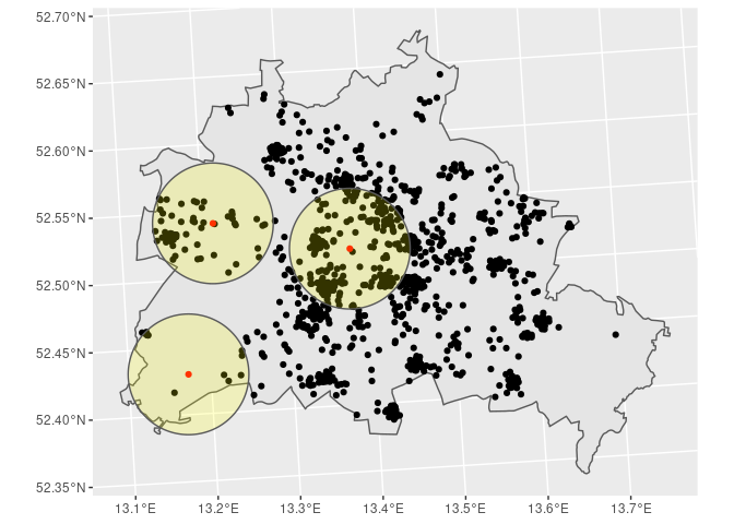
Complete Example
Suppose you want to know which households of the SOEP from survey year 2011 live within a distance of 5000m to the following points of interest (POI):
Brandenburger Tor
Zitadelle Spandau
Wannsee
Besides that, you want to know how far their distance to the corresponding POI is and which household lives closest to the corresponding POI. After computing the informations need you want to export the results for further use on the HAUSER server.
# Global stuff
# ~~~~~~~~~~~~

# packages
library(here)
library(sf)
library(tidyverse)

# global values
survey_year <- 2011
distance <- 5000 # meter
common_crs <- 25832


# Step 1: read the data
# ~~~~~~~~~~~~~~~~~~~~~

# read polygons for Federal States
States <- st_read(here('Daten', 'vg250_ebenen_0101'), layer = 'VG250_LAN', quiet = TRUE)

# read SOEP data
SOEP <- st_read(here('Daten', 'soep_v29'), quiet = TRUE)

# read POI data
POI <- st_read(here('Daten', 'POIs_Berlin.csv'), quiet = TRUE)


# Step 2: Transform data
# ~~~~~~~~~~~~~~~~~~~~~~

# transform SOEP the data
SOEP <- st_transform(SOEP, crs = common_crs)

# transform POIs
POI <- POI[, -4]

POI <- st_as_sf(POI, coords = c("X", "Y"), crs = 4326)
POI <- st_transform(POI, crs = common_crs)


# Step 3: Subset the data
# ~~~~~~~~~~~~~~~~~~~~~~~

# Berlin only
BE <- States %>%
  filter(GEN == 'Berlin')

# interesting POIs only
POI <- POI %>%
  filter(Objekt %in% c("Brandenburger Tor", "Zitadelle Spandau", "Wannsee"))

# SOEP survey year: 2011 only
SOEP <- SOEP %>%
  filter(erhebj == survey_year)

# SOEP housholds in Berlin only
SOEP <- SOEP[unlist(st_contains(BE, SOEP)), ]


# Step 4: Plot the data
# ~~~~~~~~~~~~~~~~~~~~~

BE %>%
  ggplot() + geom_sf() +
  geom_sf(data = SOEP) +
  geom_sf(data = POI, col = 'red') +
  geom_sf(data = st_buffer(POI, dist = distance),
          alpha = 0.2, fill = 'yellow')
# Step 5: Get the desired information
# ~~~~~~~~~~~~~~~~~~~~~~~~~~~~~~~~~~~
# get the household in relevant distance
soep_in_5km <- st_is_within_distance(POI, SOEP, dist = distance)
SOEP_5km <- SOEP[unlist(soep_in_5km), ]
# get the distances
dist_matrix <- as_tibble(st_distance(SOEP_5km, POI))
names(dist_matrix) <- str_c('distance_to_', str_remove(POI$Objekt, ' '))
# attach distances to data
SOEP_5km <- bind_cols(SOEP_5km, dist_matrix)
# find the nearest household
nearest_hh <- st_nearest_feature(POI, SOEP_5km)
SOEP_5km$nearest_to <- ''
SOEP_5km$nearest_to[nearest_hh] <- POI$Objekt
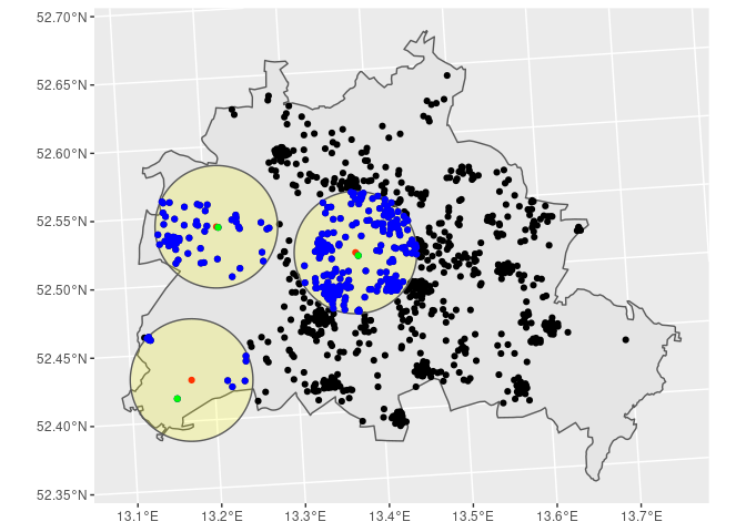
# Step 6: Check your data
# ~~~~~~~~~~~~~~~~~~~~~~~
BE %>%
ggplot() + geom_sf() +
geom_sf(data = SOEP) +
geom_sf(data = POI, col = 'red') +
geom_sf(data = st_buffer(POI, dist = distance),
alpha = 0.2, fill = 'yellow') +
geom_sf(data = SOEP_5km, col = 'blue') +
geom_sf(data = SOEP_5km[SOEP_5km$nearest_to != '', ], col = 'green')
# Step 7: Export your data
# ~~~~~~~~~~~~~~~~~~~~~~~~
path_export <- paste0('/home/', Sys.info()['user'], '/transfer/export/',  Sys.Date())

if(!file.exists(path_export)){
  dir.create(path_export, recursive = TRUE)
}

st_write(SOEP_5km, file.path(path_export, 'Output.csv'),
         append = FALSE, overwrite = TRUE)
## Deleting layer `Output' using driver `CSV'
## Writing layer `Output' to data source `/home/hwsteinhauer/transfer/export/2021-01-27/Output.csv' using driver `CSV'
## Updating existing layer Output
## Writing 356 features with 6 fields and geometry type Point.
README <- tibble(name = names(SOEP_5km)[-grep('geometry', names(SOEP_5km))],
                 description = c('erhebj',
                                 'ID',
                                 'distance (in meters) of household to Brandenburger Tor',
                                 'distance (in meters) of household to Wannsee',
                                 'distance (in meters) of household to Zitadelle Spandau',
                                 'household nearest to the POI'))

write.csv(README, file.path(path_export, 'README.csv'),
         row.names = FALSE)
Appendix
Session info - Platform
##  setting  value
##  version  R version 4.0.3 (2020-10-10)
##  os       Ubuntu 20.04.1 LTS
##  system   x86_64, linux-gnu
##  ui       X11
##  language (EN)
##  collate  de_DE.UTF-8
##  ctype    de_DE.UTF-8
##  tz       Europe/Berlin
##  date     2021-01-27
Session info - Packages
##  package     * version date       lib source
##  bookdown    * 0.21    2020-10-13 [1] CRAN (R 4.0.3)
##  dplyr       * 1.0.2   2020-08-18 [1] CRAN (R 4.0.2)
##  forcats     * 0.5.0   2020-03-01 [1] CRAN (R 4.0.0)
##  ggplot2     * 3.3.2   2020-06-19 [1] CRAN (R 4.0.1)
##  gridExtra   * 2.3     2017-09-09 [1] CRAN (R 4.0.0)
##  here        * 1.0.0   2020-11-15 [1] CRAN (R 4.0.3)
##  kableExtra  * 1.3.1   2020-10-22 [1] CRAN (R 4.0.3)
##  knitr       * 1.30    2020-09-22 [1] CRAN (R 4.0.2)
##  pacman      * 0.5.1   2019-03-11 [1] CRAN (R 4.0.2)
##  purrr       * 0.3.4   2020-04-17 [1] CRAN (R 4.0.0)
##  readr       * 1.4.0   2020-10-05 [1] CRAN (R 4.0.3)
##  rgdal       * 1.5-19  2021-01-05 [1] CRAN (R 4.0.3)
##  sessioninfo * 1.1.1   2018-11-05 [1] CRAN (R 4.0.0)
##  sf          * 0.9-7   2021-01-06 [1] CRAN (R 4.0.3)
##  sp          * 1.4-4   2020-10-07 [1] CRAN (R 4.0.3)
##  stringr     * 1.4.0   2019-02-10 [1] CRAN (R 4.0.0)
##  tibble      * 3.0.4   2020-10-12 [1] CRAN (R 4.0.3)
##  tidyr       * 1.1.2   2020-08-27 [1] CRAN (R 4.0.2)
##  tidyverse   * 1.3.0   2019-11-21 [1] CRAN (R 4.0.0)
##
## [1] /home/hwsteinhauer/R/x86_64-pc-linux-gnu-library/4.0
## [2] /usr/local/lib/R/site-library
## [3] /usr/lib/R/site-library
## [4] /usr/lib/R/library
Section author: Hans Walter Steinhauer hwsteinhauer@diw.de
Last updated: 2021-02-22